Gator: Cross-view Jigsaw Objective for Self-Supervised 3D Vision

Self-supervised learning has become a standard paradigm for learning visual representations from unlabeled data. Methods such as DINO [3] and MAE [4] achieve strong results through self-distillation and masked image reconstruction, respectively. Masked modeling has further been extended to two-view pretraining with CroCo [2], and even multi-view modeling by MuM [11], both exhibting strong performance on 3D vision tasks.

Another successful self-supervised paradigm for one-view models is jigsaw puzzle solving [5], where the pretraining goal consists in reordering shuffled patches of the input image. This method has proven effective for several applications, like video understanding [8] and multimodal LLMs [10] Yet, its use as a pretraining method for multi-view modeling remains largely unexplored. In this work, we investigate whether a two-view jigsaw objective can serve as an effective pretraining strategy for 3D tasks such as image matching and optical flow.

In this work we present Gator, a new self-supervised method based on jigsaw solving for multi-view models. During pretraining, the model recieves two views of the same scene: we keep one view unchanged and shuffle the patches of the other. The model is trained to recover the correct patch arrangement by exploiting the reference view, thereby encouraging the learning of spatial structure and cross-view correspondences. Our approach is not formulated as pixel-level prediction: instead, it formulates the pretraining objective as a patch reordering problem. This objective still requires 3D understanding to be solved, but without using model parameters for low-level detail reconstruction such as textures. We also compare our model after finetuning on several downstream tasks against one-view and multi-view methods, showing that Gator achieves competitive results in 3D vision downstream tasks.

Jigsaw puzzle solving has been widely studied as a self-supervised pretext task for visual representation learning. The main idea is to shuffle image patches and train the model to recover their original spatial arrangement, encouraging the representation to capture spatial layout rather than only local appearance. This idea has been explored in both convolutional models and Vision Transformers, including Jigsaw-ViT, where the patch-based structure of ViTs makes the jigsaw objective a natural fit [5], [6]. However, these methods are mainly single-view: they learn spatial structure within one image, but they are not explicitly trained to reason across two different views of the same scene.

Cross-view pretraining is especially important for 3D vision, where downstream tasks often require geometric reasoning between image pairs. CroCo is the closest work to ours in this setting [2]. It receives a clean reference image and a masked target image, and learns to reconstruct the missing target patches by using information from both views. This objective encourages the model to learn scene structure and cross-view correspondences. Gator follows the same cross-view motivation, but replaces masked pixel reconstruction with patch-order prediction. In this way, the model is trained to use the reference view to solve a jigsaw task, focusing the pretraining signal on spatial organization and correspondence reasoning rather than low-level pixel recovery.

III-A. Architecture

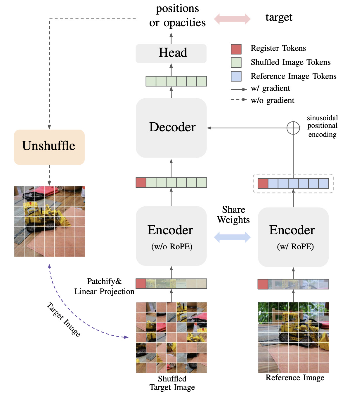
Gator follows an encoder-decoder architecture. The encoder is equivalent to ViT-Small, consisting of 12 layers, a hidden dimension of 384, and 6 attention heads. The decoder is a 6-layer Transformer with the same hidden dimension and number of attention heads as the encoder. Following [1], we add four learnable register tokens.
Two different views of the same scene are passed to the model: one view, called shuffled, contains shuffled patches of size 16×16, while the other view is used as the reference. The model predicts how to reorder the shuffled view so that it matches the reference view.
We first patchify both views and linearly project the resulting patch tokens to the hidden dimension. We then concatenate the register tokens with the patch tokens and process both views using the same encoder. For the shuffled view, we disable RoPE in the encoder to prevent the model from inferring positional information directly from the RoPE coefficients.
The decoder then processes the shuffled-view tokens as queries and the reference-view tokens as context. We add sinusoidal positional embeddings to the reference-view tokens instead of using RoPE, since tokens at the same positions in the two views may correspond to different 3D locations.
Finally, the output head processes each token independently and predicts either a position, represented as logits or a 2D coordinate, or opacity, depending on the loss function used. We experiment with four different losses, which are described below.

III-B. Jigsaw Objectives

Let the input image have size \(N \times N \times C\), and let the patch size be \(p\). This yields an \(n \times n\) patch grid, where \(n = N / p\). In the description below, we use 2D grid positions and their corresponding 1D indices in the flattened grid interchangeably for simplicity.

Classification Loss. A linear head maps each token representation to logits over all possible patch positions: \[ \hat{y}_k = W h_k + b, \qquad \hat{y}_k \in \mathbb{R}^{n^2}. \] For token \(k\), the target \(y_k\) is the index of its true position in the grid. We train the model using cross-entropy loss against the true position. At inference time, we recover the predicted position by taking \(\arg\max_j \hat{y}_{k,j}\). \[ \mathcal{L}_1 = \operatorname{CrossEntropy}(\hat{y}_k, y_k). \]

Distance-Based Loss. A linear head maps each token representation to a normalized 2D coordinate: \[ \hat{u}_k = \tanh(W h_k + b), \qquad \hat{u}_k \in [-1, 1]^2. \] The target coordinate \(u_k\) is the normalized true position of the patch. We train the model using mean squared error against the target coordinate. To recover a discrete position, we map predictions from \([-1,1]\) to \([0,n-1]\) and round each coordinate to the nearest integer. \[ \mathcal{L}_2 = \operatorname{MSE}(\hat{u}_k, u_k). \]

Visual Loss. A linear head maps each token representation to \(n^2\) values, followed by a softmax: \[ o_k = \operatorname{softmax}(W h_k + b), \qquad o_k \in \mathbb{R}^{n^2}. \] Here, \(o_{k,i}\) denotes the predicted opacity for placing patch \(k\) at position \(i\). Let \(z_k \in \mathbb{R}^{p^2 C}\) be the flattened ground-truth patch corresponding to token \(k\). We softly place each patch at all possible positions and sum over patches: \[ \hat{Z}_i = \sum_{k=1}^{n^2} o_{k,i} z_k, \qquad \hat{Z} = \{\hat{Z}_1, \dots, \hat{Z}_{n^2}\}, \qquad \hat{Z} \in \mathbb{R}^{n^2 \times p^2 C}. \] The loss is the mean squared error between the reconstructed patchified image \(\hat{Z}\) and the ground-truth patchified image \(Z\): \[ \mathcal{L}_3 = \operatorname{MSE}(\hat{Z}, Z). \] This objective naturally handles cases in which visually identical patches are swapped, since such swaps do not increase the reconstruction error.

Similarity Loss. This loss combines ideas from the classification and visual losses. As in the classification loss, a linear head maps each token representation to logits over all patch positions: \[ \hat{y}_k = W h_k + b, \qquad \hat{y}_k \in \mathbb{R}^{n^2}. \] However, instead of penalizing all incorrect positions equally, we allow the model to assign probability mass to visually similar patches. For token \(k\), we define a soft target distribution over positions as \[ q_k^j = \operatorname{softmax}_j \left( -\frac{\lVert z_k - z_j \rVert_2^2}{\tau p^2 C} \right), \] where \(\tau\) is a temperature hyperparameter and \(p^2 C\) normalizes by the patch dimensionality. The model is then trained with cross-entropy against this target distribution: \[ \mathcal{L}_4 = \operatorname{CrossEntropy}(\hat{y}_k, q_k). \]

III-C. Pre-training Details

Due to the permutation invariance of the Transformer architecture, we do not explicitly shuffle the patches of the shuffled view during training, but pass them as they are. Since no positional information is provided for this view, omitting the explicit shuffle does not simplify the task.

Our experiments with the Single View Jigsaw model suggest that strong jigsaw solving performance can be achieved without relying on the reference view. However, the reference view is crucial for strong 3D performance, and therefore our model must learn to use it effectively. To encourage this behavior, we randomly mask between 35% and 85% of the shuffled-view patches during training. As a result, the model cannot rely solely on the shuffled view and must instead learn to use the reference view to solve the task. In the appendix (sec B), we show that this strategy effectively encourages the model to utilize the reference view.

IV-A. Optimization Details

Following CroCo [2], we render approximately 1.8M image pairs. We split the dataset into 181 shards and randomly allocate 177 shards for training and 4 shards for validation. Sharding improves GPU utilization from 60% to 90%.

We train our model and all competitors on this dataset using a fixed compute budget of 24 hours on a single V100 GPU. We tune the learning rates of CroCo, Jigsaw, and Gator on the validation set according to pre-training task performance. We use a learning rate of \(1.5 \cdot 10^{-4}\) for CroCo, \(10^{-4}\) for Gator-Classification and Jigsaw, and \(3 \cdot 10^{-4}\) for Gator-Distance-Based. We use \(\texttt{AdamW}\) with a weight decay of \(5 \cdot 10^{-2}\) for CroCo and \(10^{-2}\) for the other models. All models are trained with a batch size of 128 and a patch size of 16. We use a cosine learning rate schedule with one warm-up epoch. Training is performed in \(\texttt{fp16}\) precision with FlashAttention.

IV-B. Jigsaw Solving

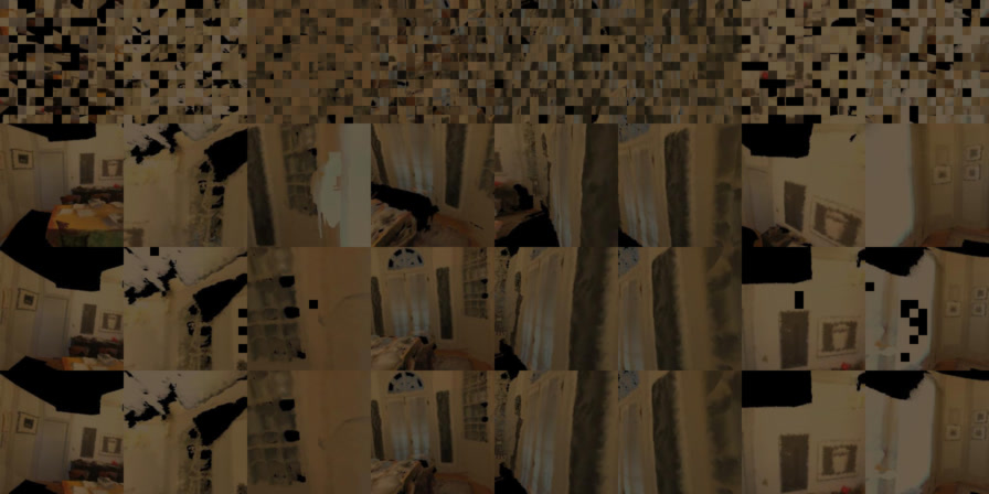
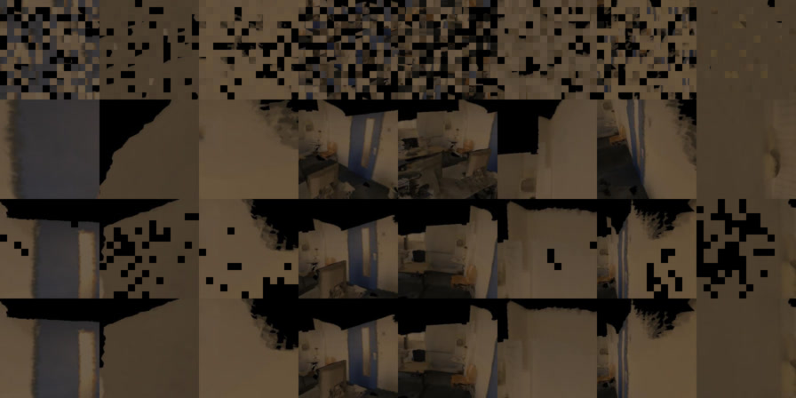
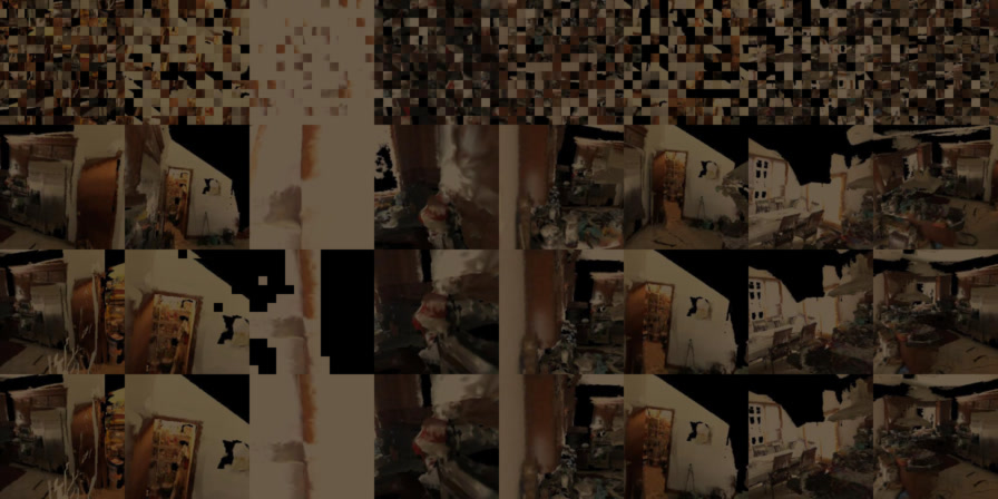
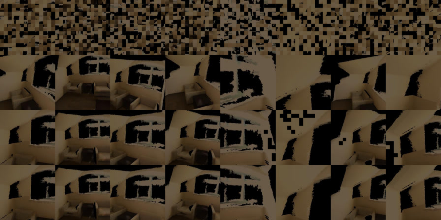
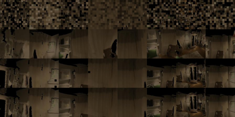
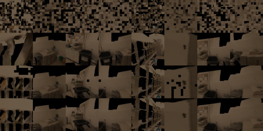
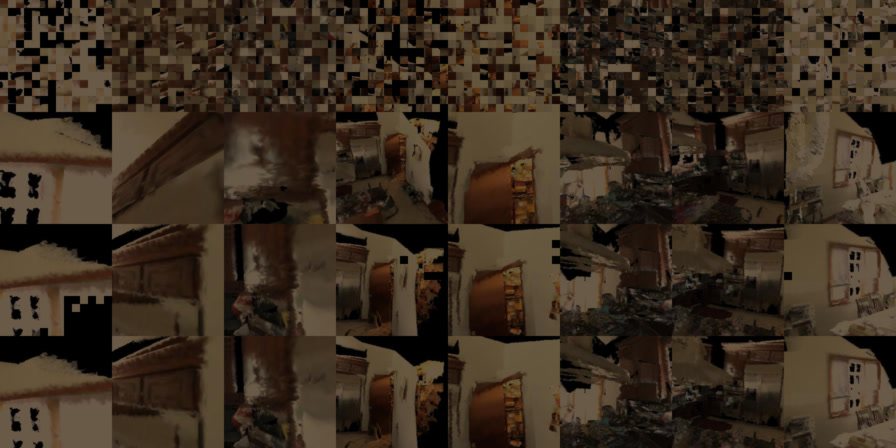
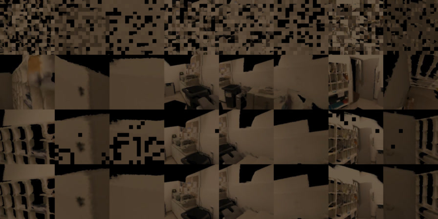
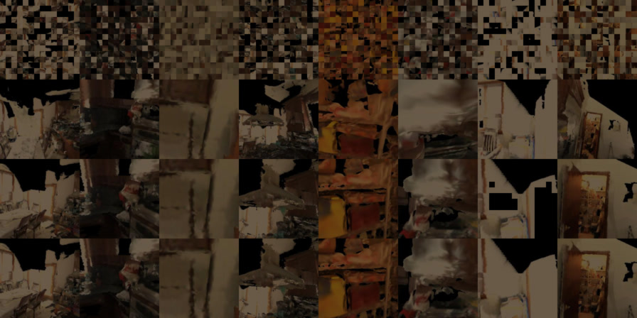
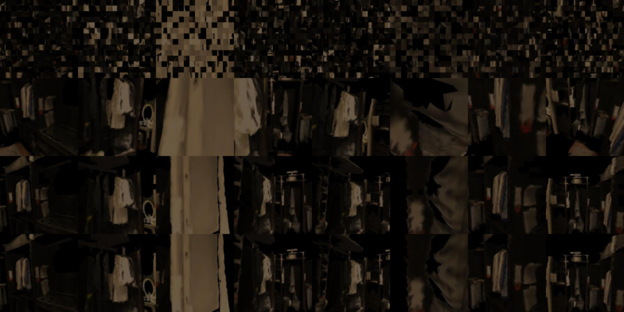
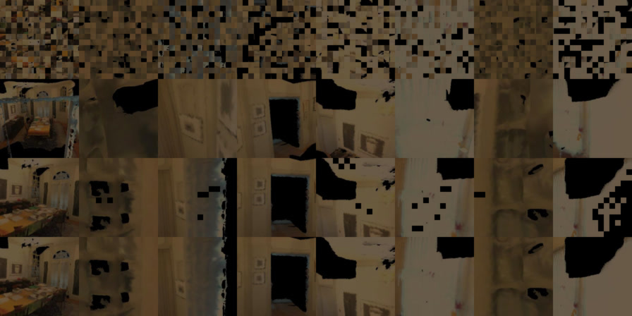
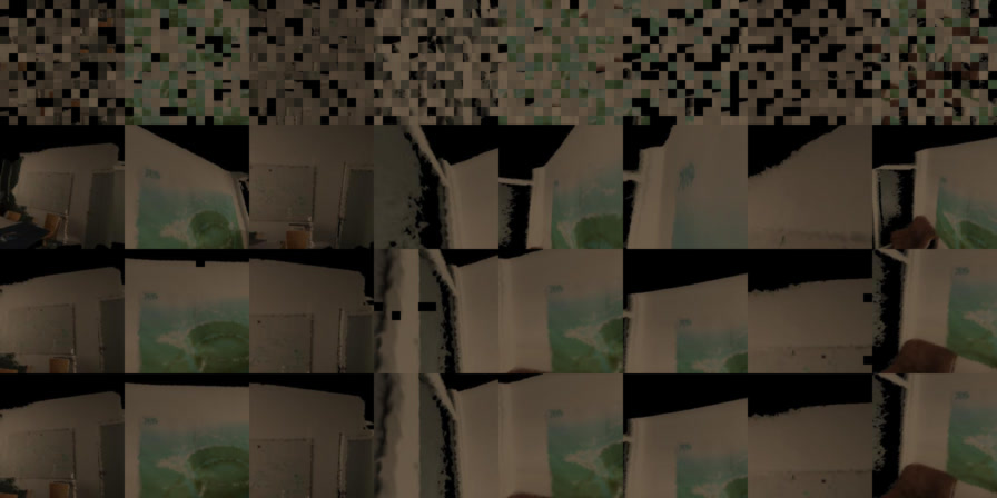
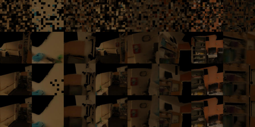
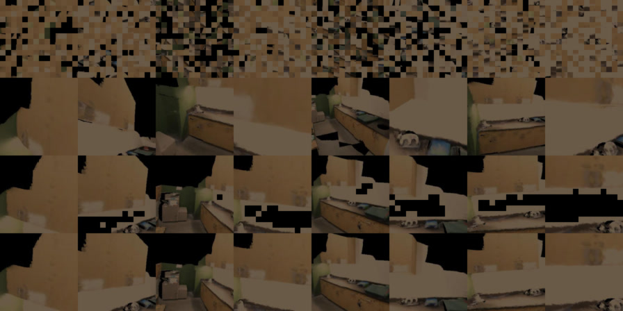
The picture is a carousel. Tap to activate scrolling. The first row shows the shuffled view, the second row shows the reference view, the third row shows the reshuffling using predicted positions, and the last row shows the ground truth image.

The model achieves an accuracy of 88.9% in predicting the true patch positions. Examples of the model's predictions are shown in the carousel above. The Jigsaw model achieves an accuracy of 88.2%, which is slightly lower than Gator but remains competitive. This result suggests that, even without using the reference view, the model can solve jigsaw puzzles to a large extent. It also highlights the need to encourage the model to rely on the reference view in order to learn representations efficient for downstream 3D tasks.

IV-C. Classification

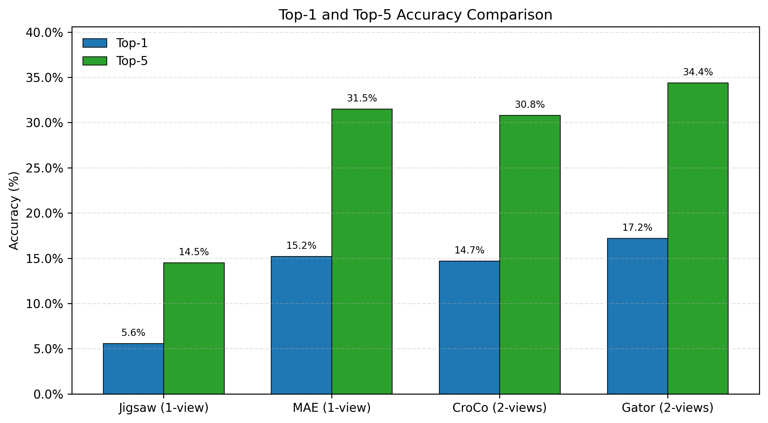
We evaluate representation quality via linear probing on ImageNet-1k: the backbone is frozen and a single linear head is trained on top of the extracted features. All models are trained with Adam, learning rate $10^{-3}$, cosine decay with 10% warm-up, batch size 512, for 25 epochs. We obtained the following results:

The low absolute accuracy reflects the significant domain gap between the pre-training data (Habitat indoor scenes) and ImageNet. Despite this gap, Gator-Small consistently outperforms all baselines, confirming that the cross-view jigsaw objective yields more transferable representations than pixel-level reconstruction (CroCo) or single-view objectives (MAE, Jigsaw). Classification examples are provided in App. C

IV-D. Optical Flow

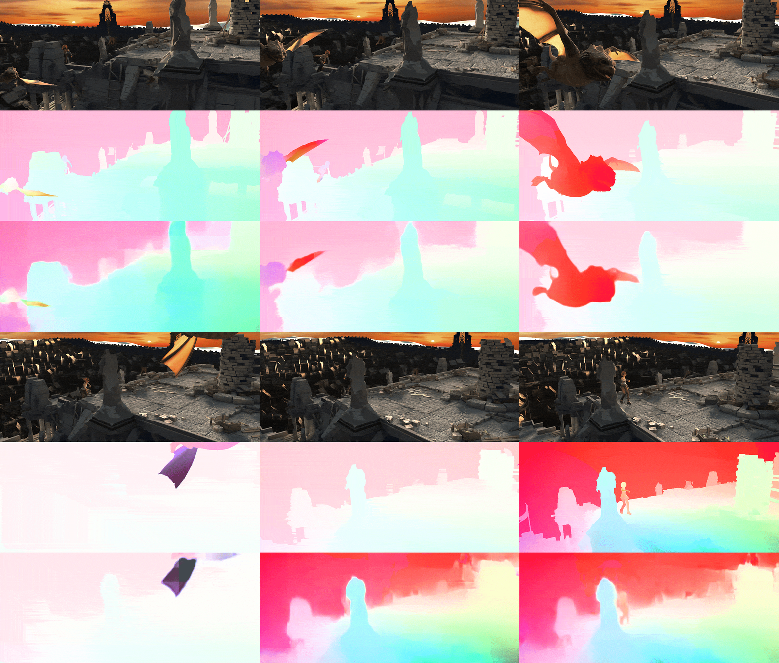
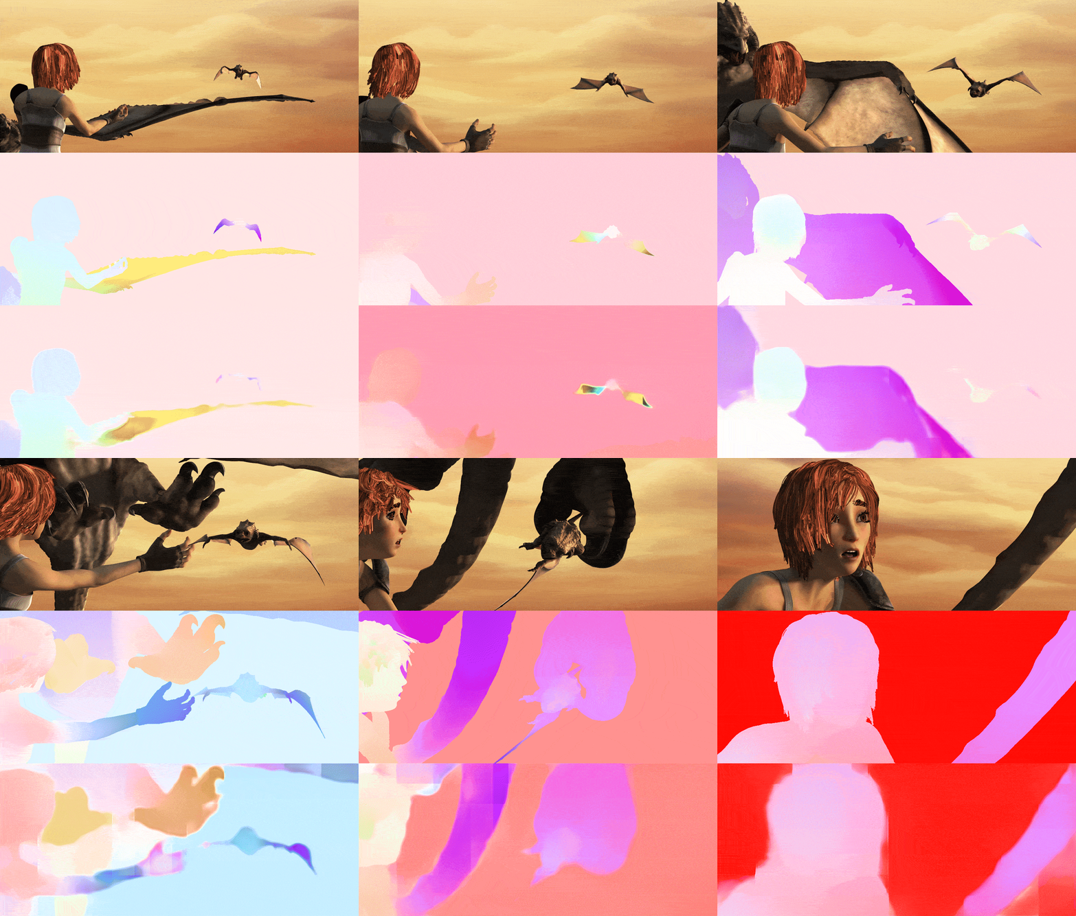
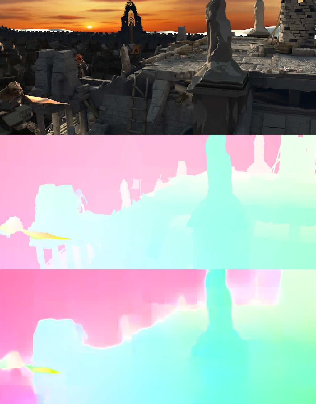
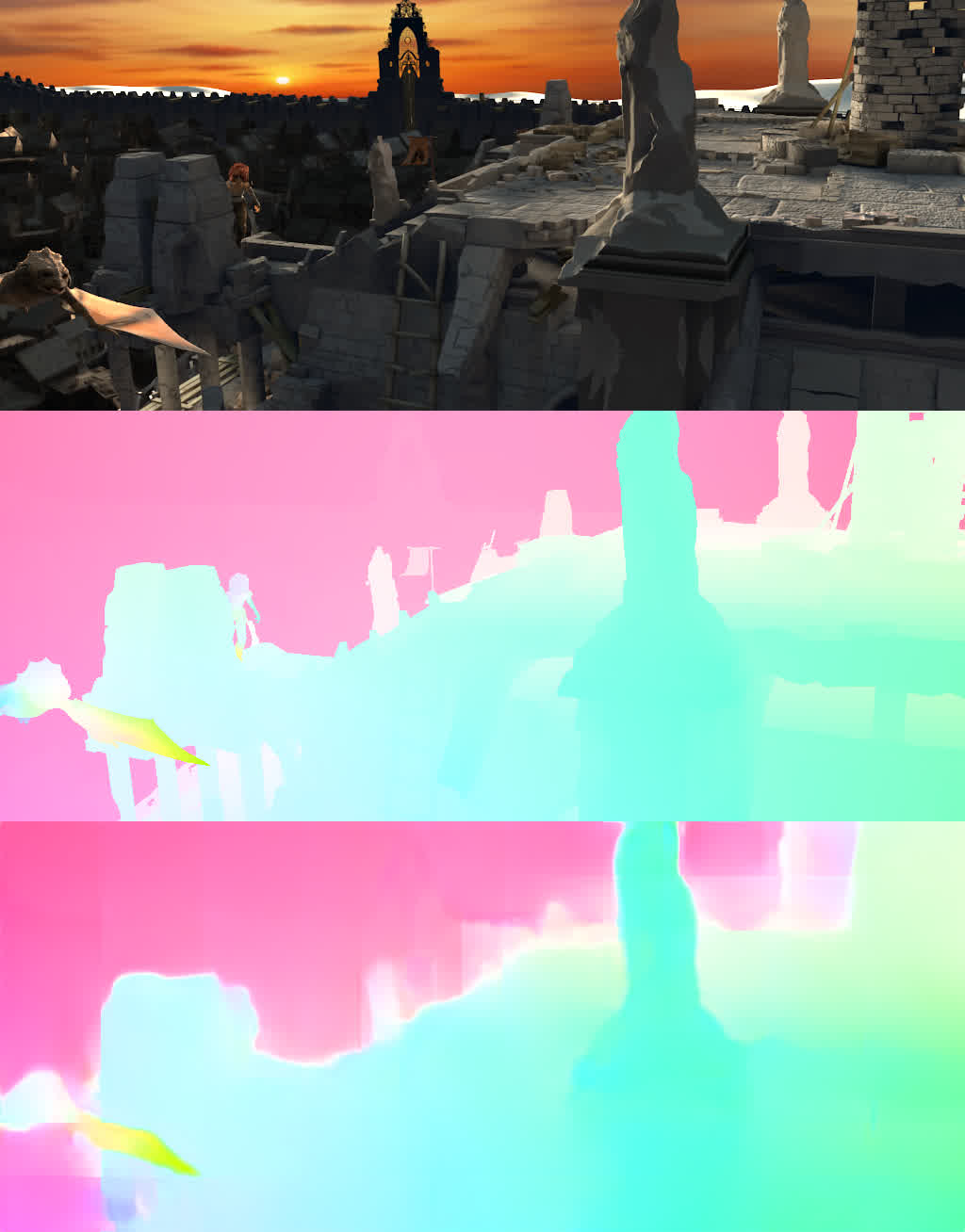
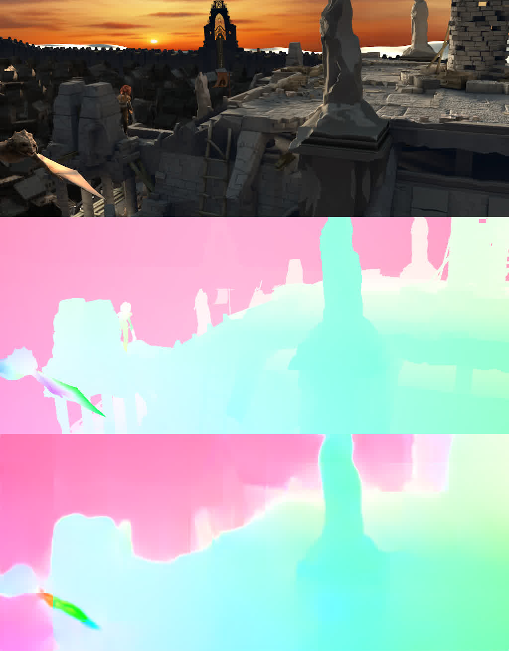
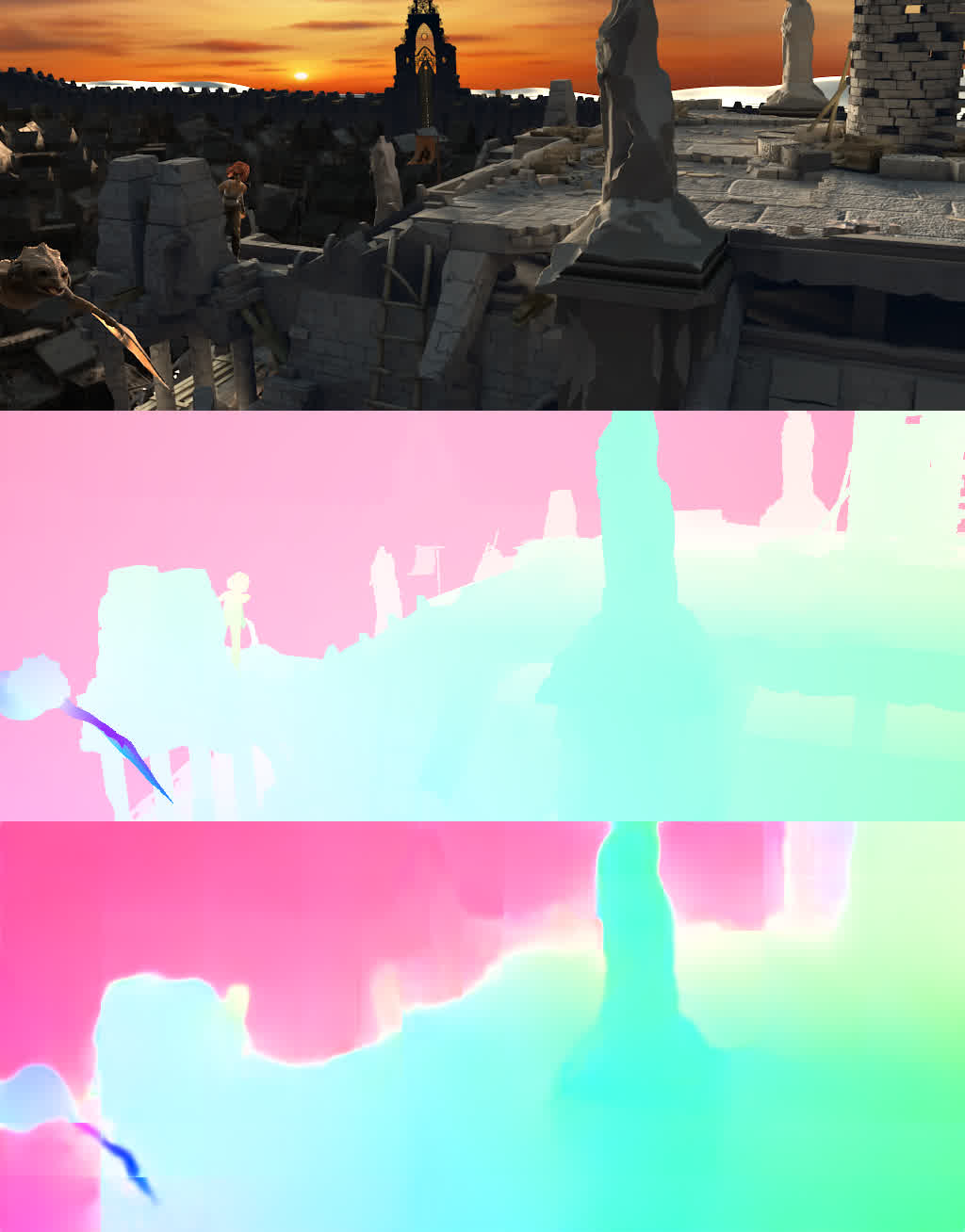
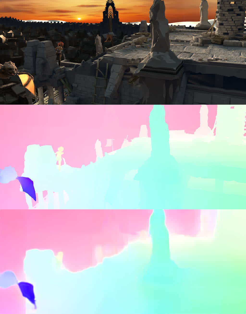
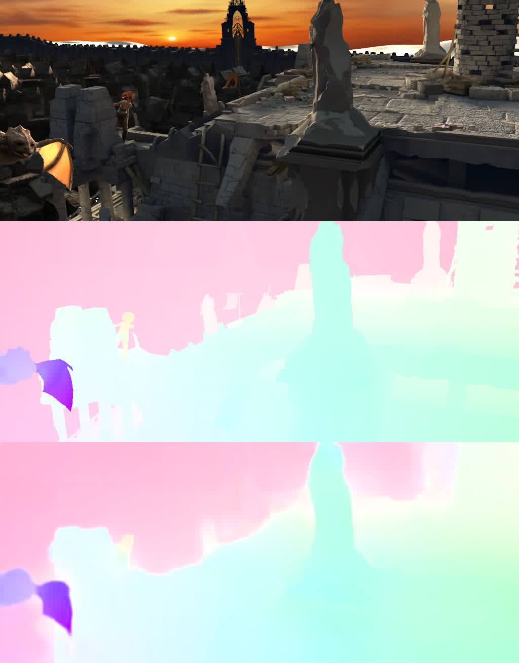
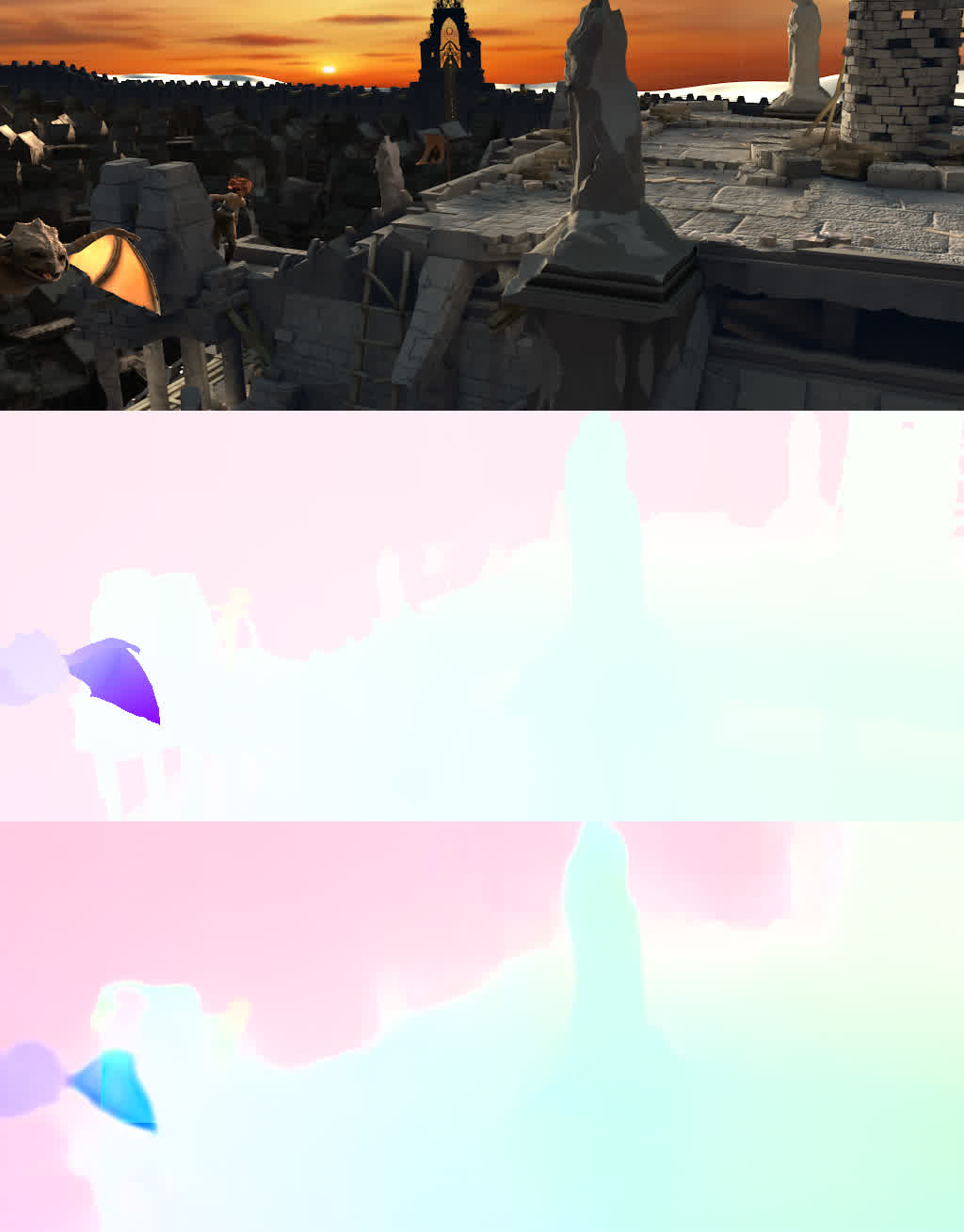
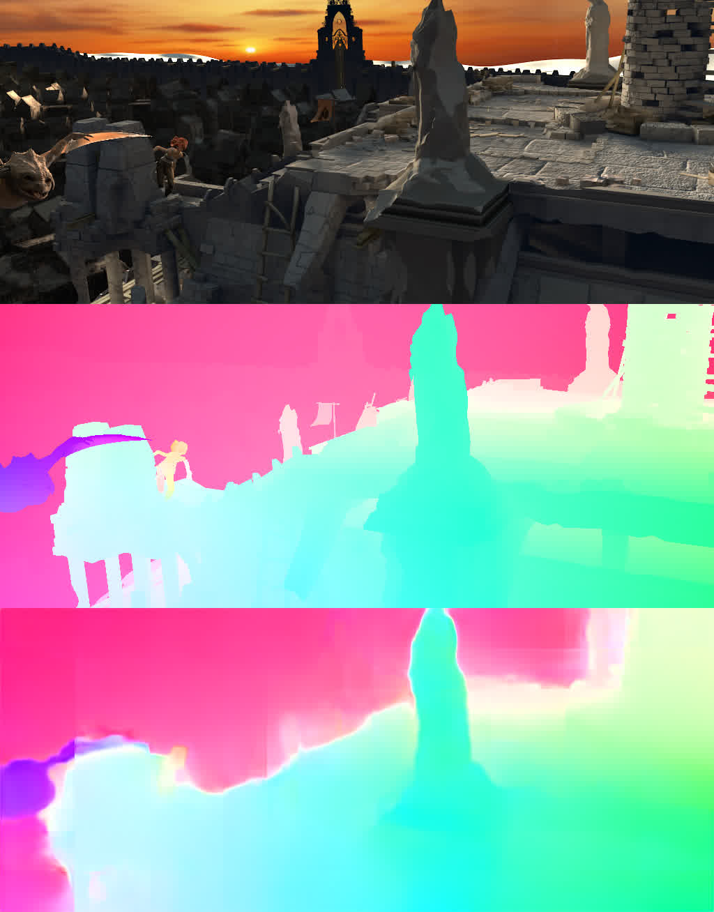
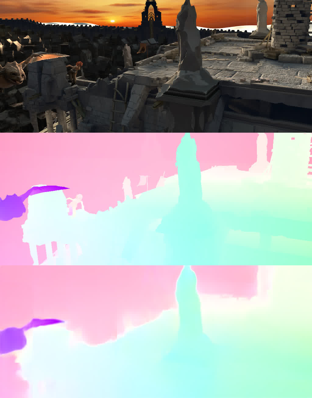
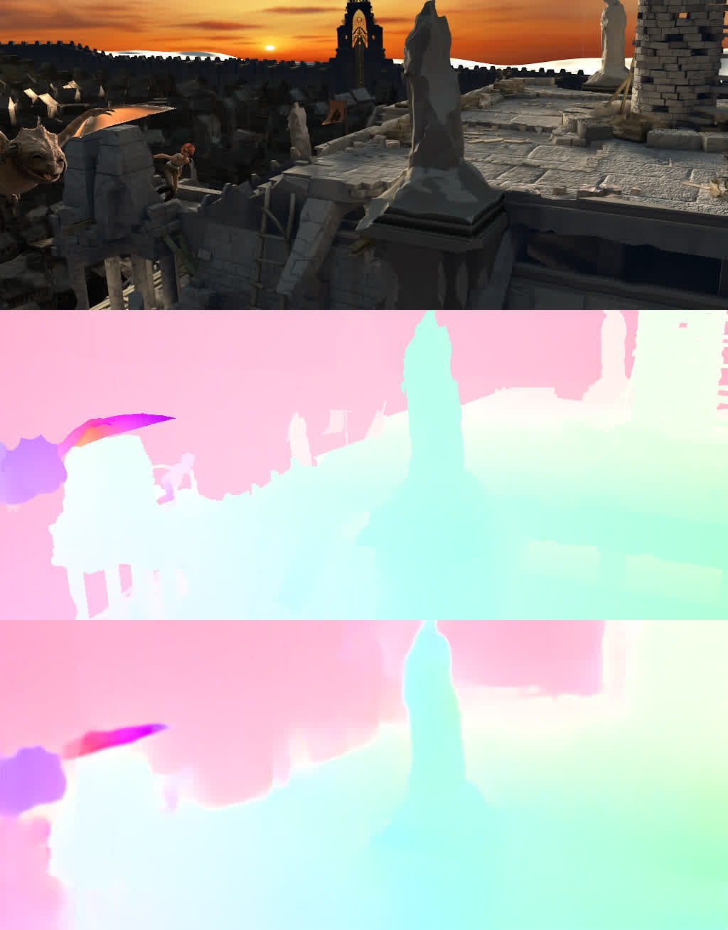
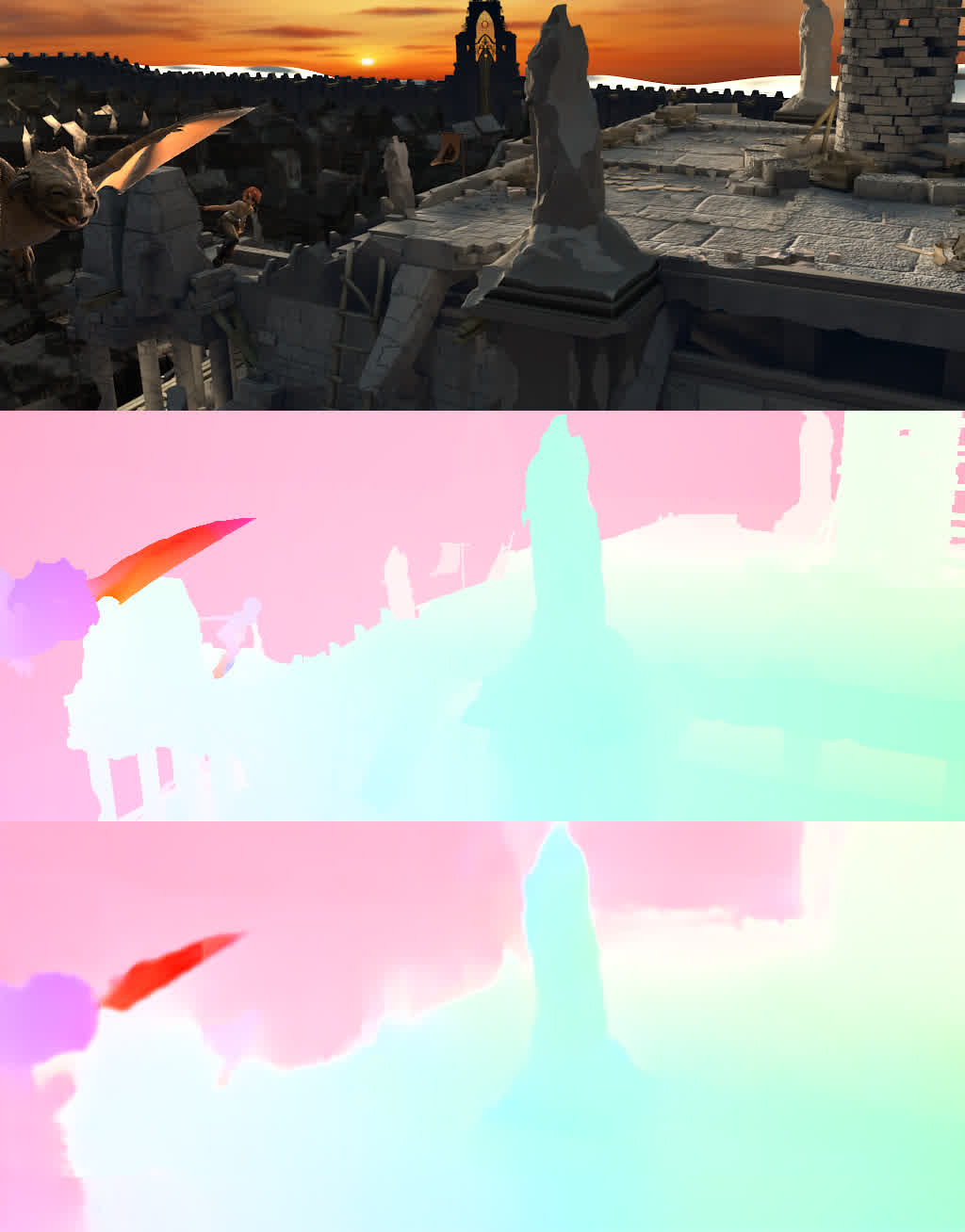
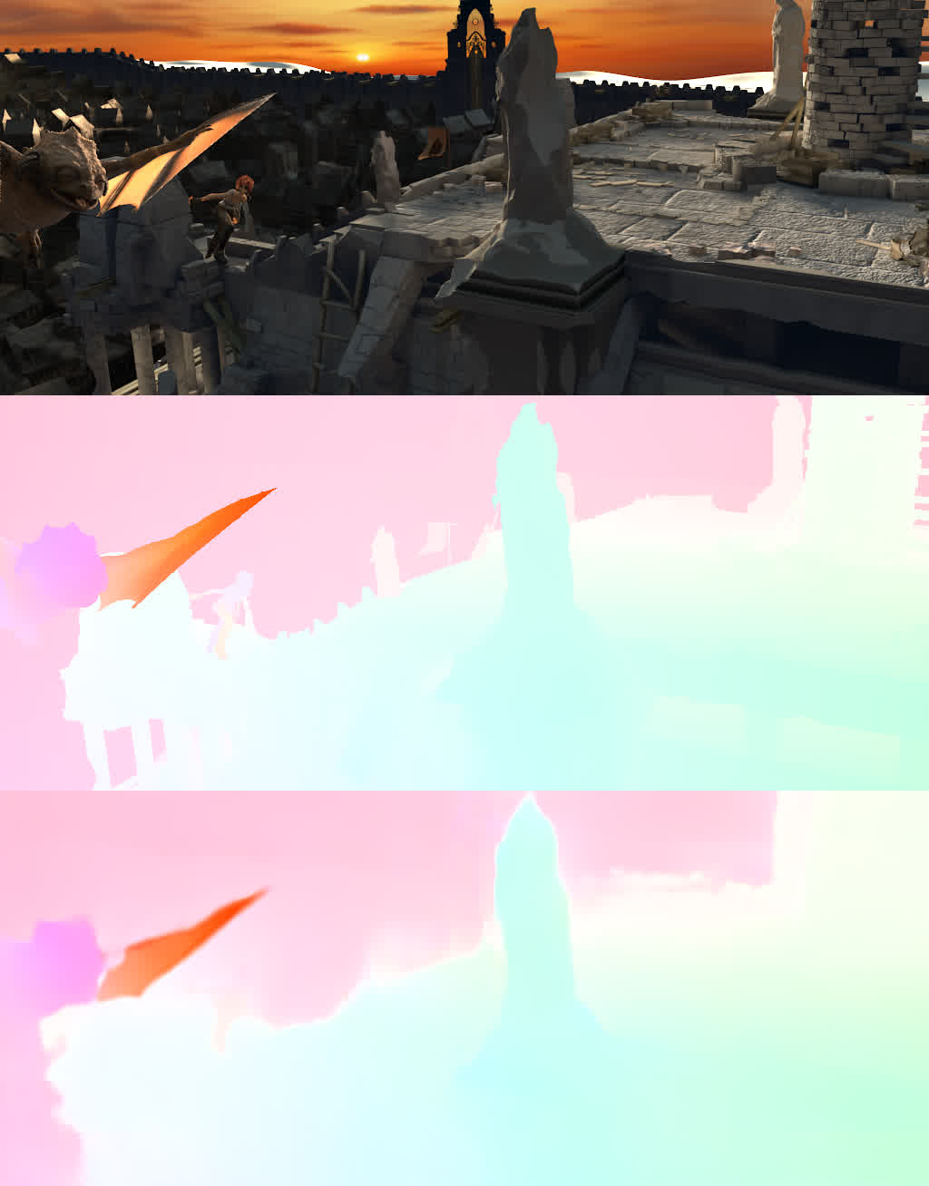
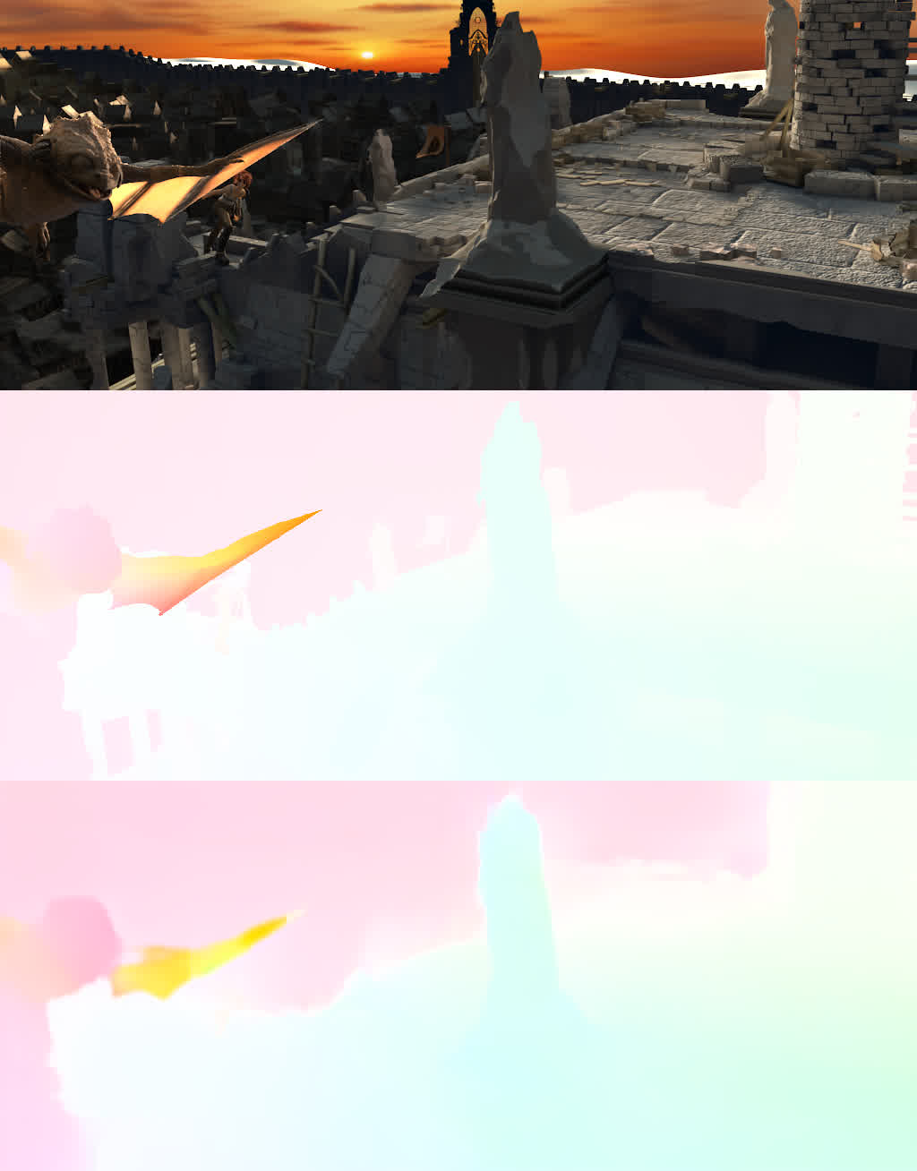
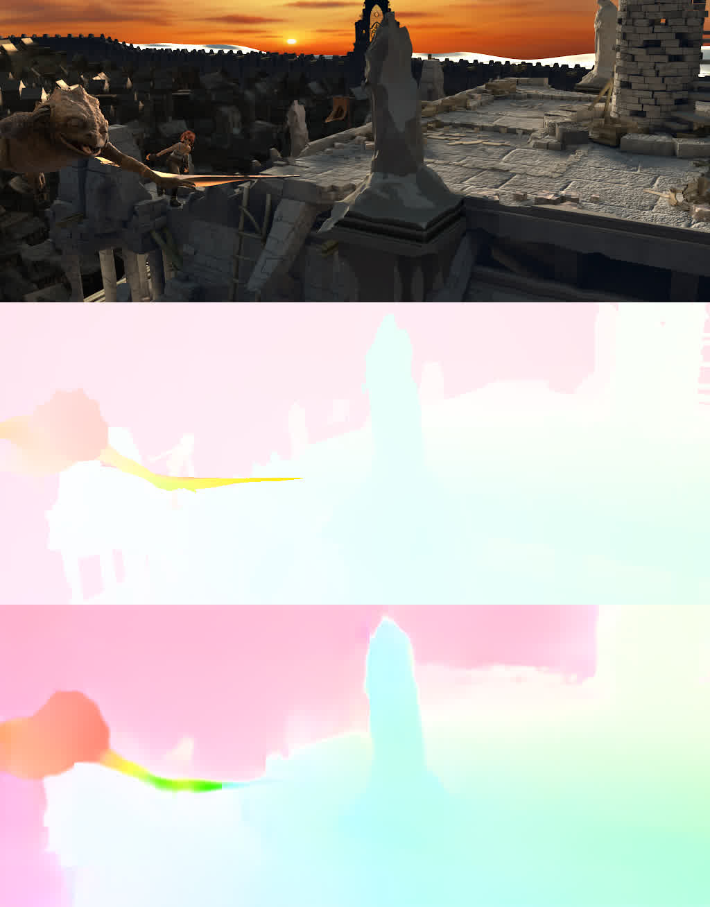
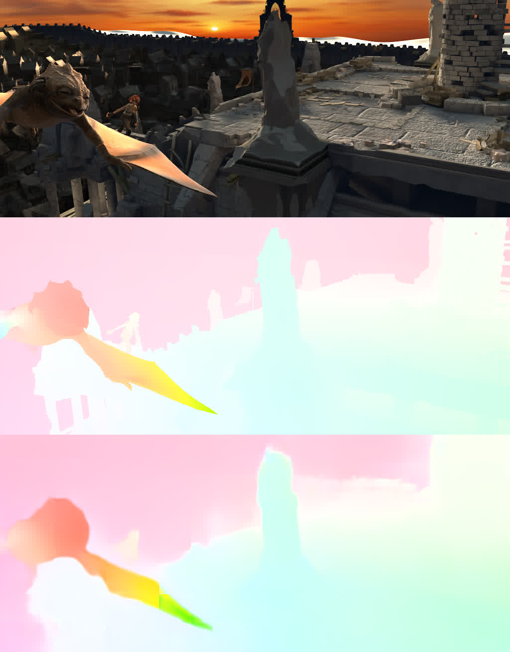
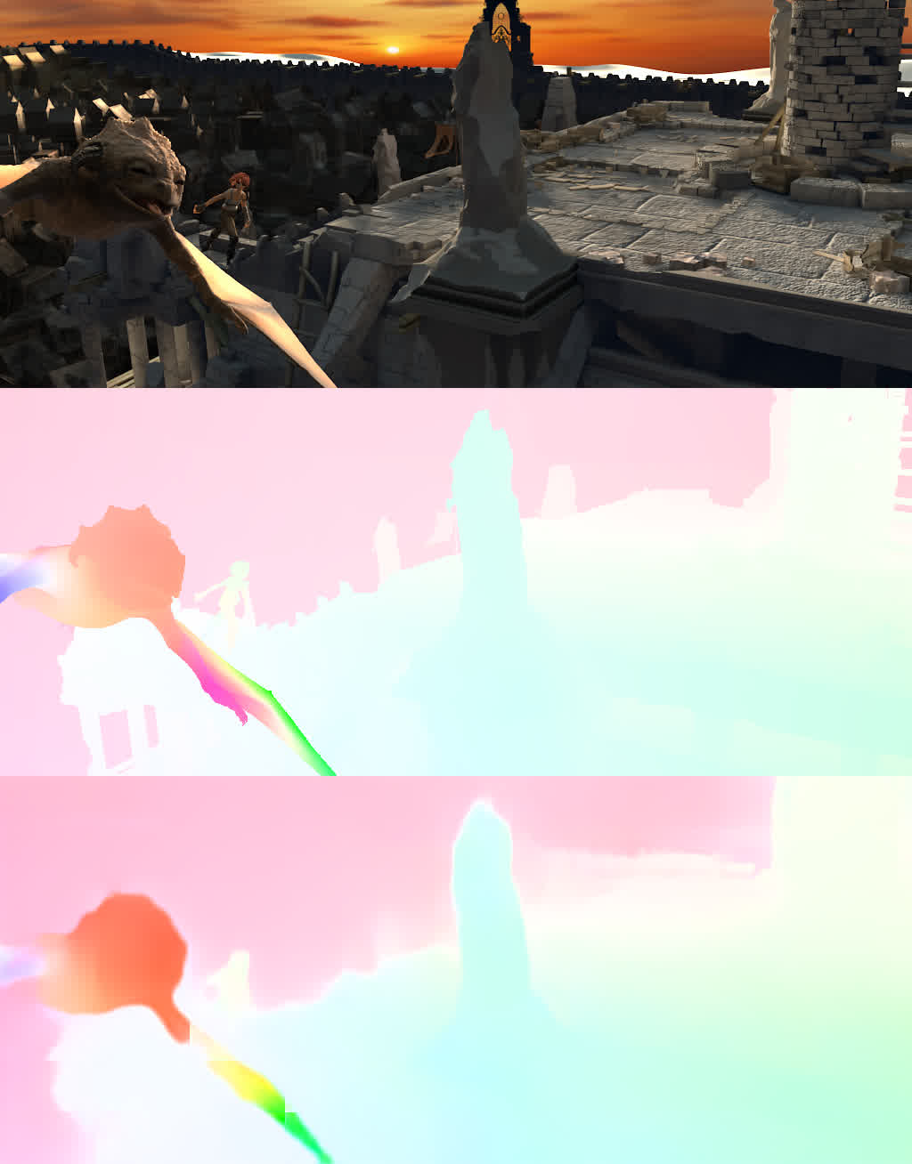
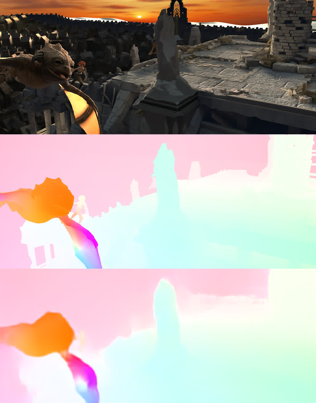
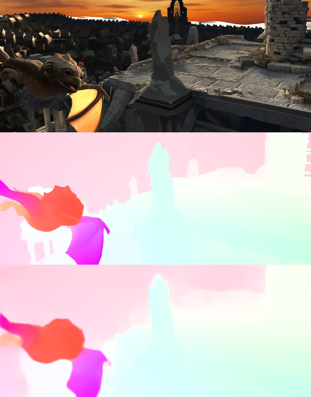
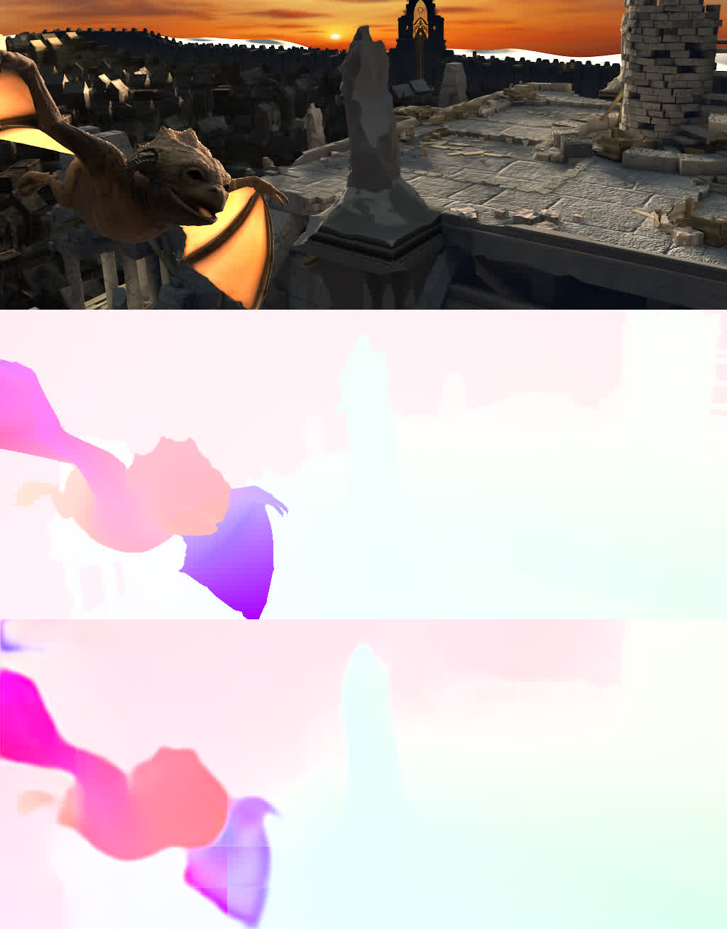
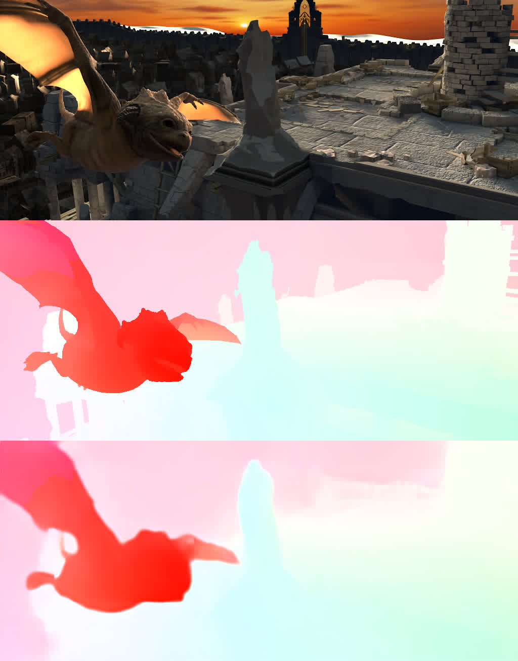
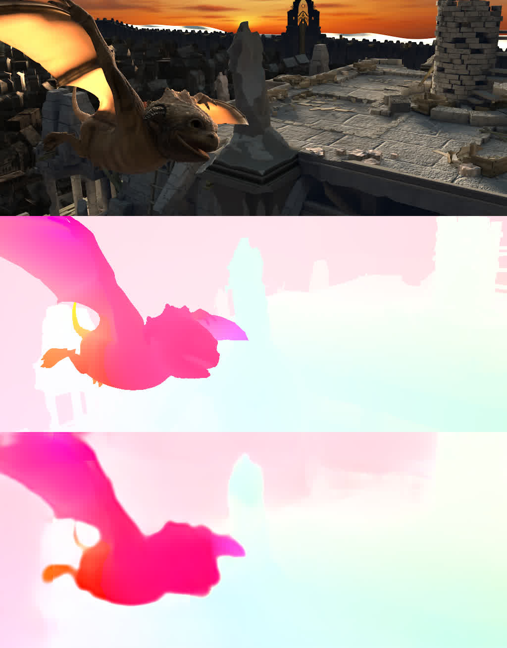
Optical flow requires to predict a 2D dense vector field assigning a displacement value to every pixel, taking as input two consecutive frames of a scene in motion. For reference, we show an input example, alongside with the ground truth prediction and the Gator prediction. To demostrate the quality of the predictions, we show two gifs with the results obtained on two different scenes of the MPI-Sintel dataset. More examples of optical flow predictions are provided in App. D.

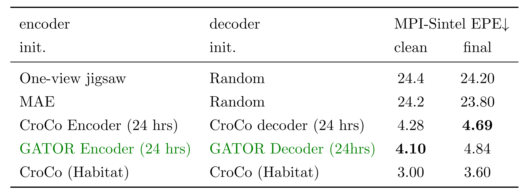
The following table shows the results obtained by finetuning the models on the MPI-Sintel + FlyingChairs datasets for 50 epochs. The reported performance refers to the MPI-Sintel test set, which contains frames from two different scenes unseen during training.

The results show that Gator reaches comparable performance with CroCo, using the same compute. This results show the effectiveness of Gator's representations and their efficient transferability to this task.
For reference, in the last row of the table we report the results from the original CroCo paper: their model is a ViT-base, pretrained for 2 weeks using four V100 and finetuned on a different dataset. Therefore, we include its performance in the table for a complete overview, even if the comparison with the other models is not fair.

IV-E. Relative Pose Regression

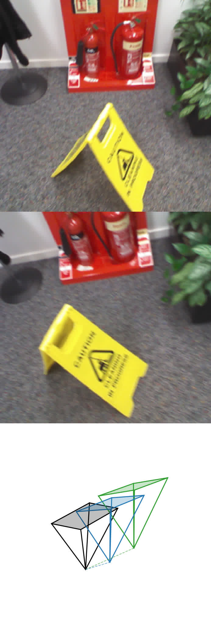
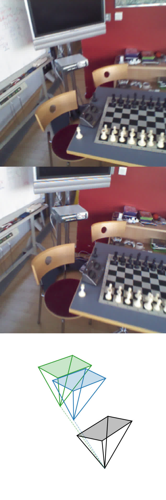
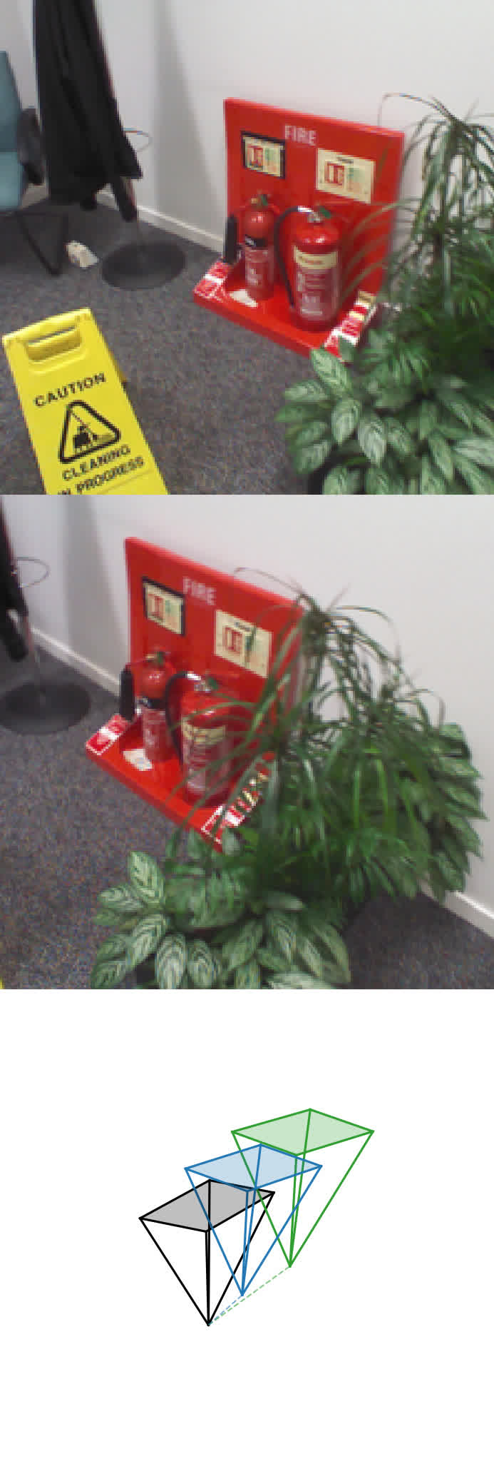
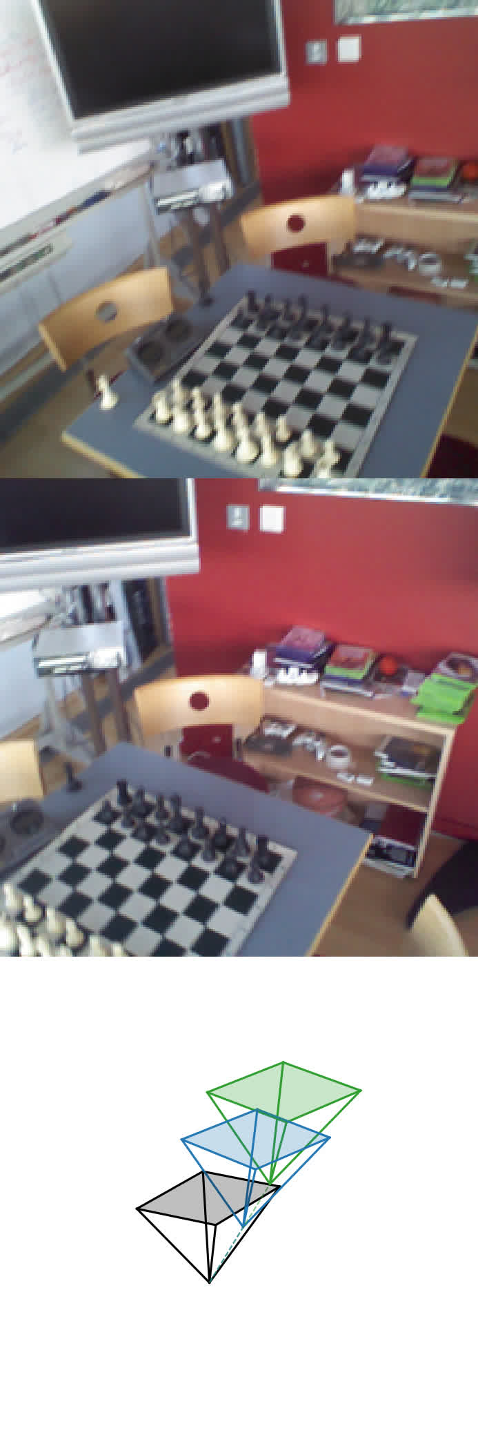
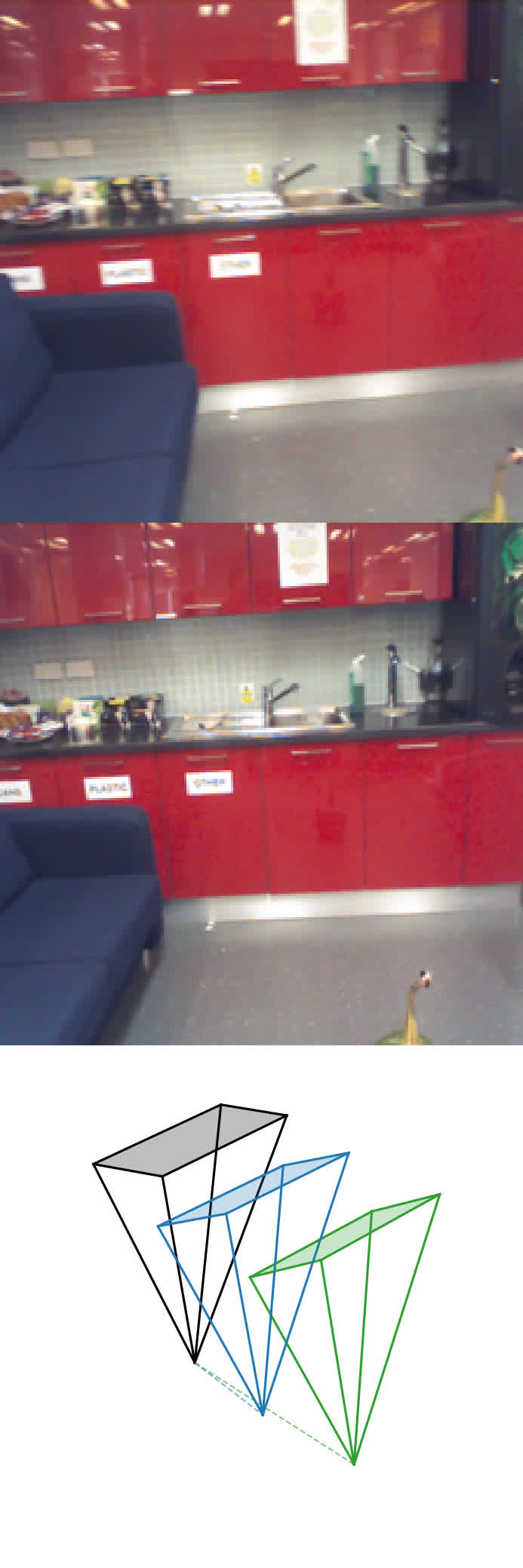
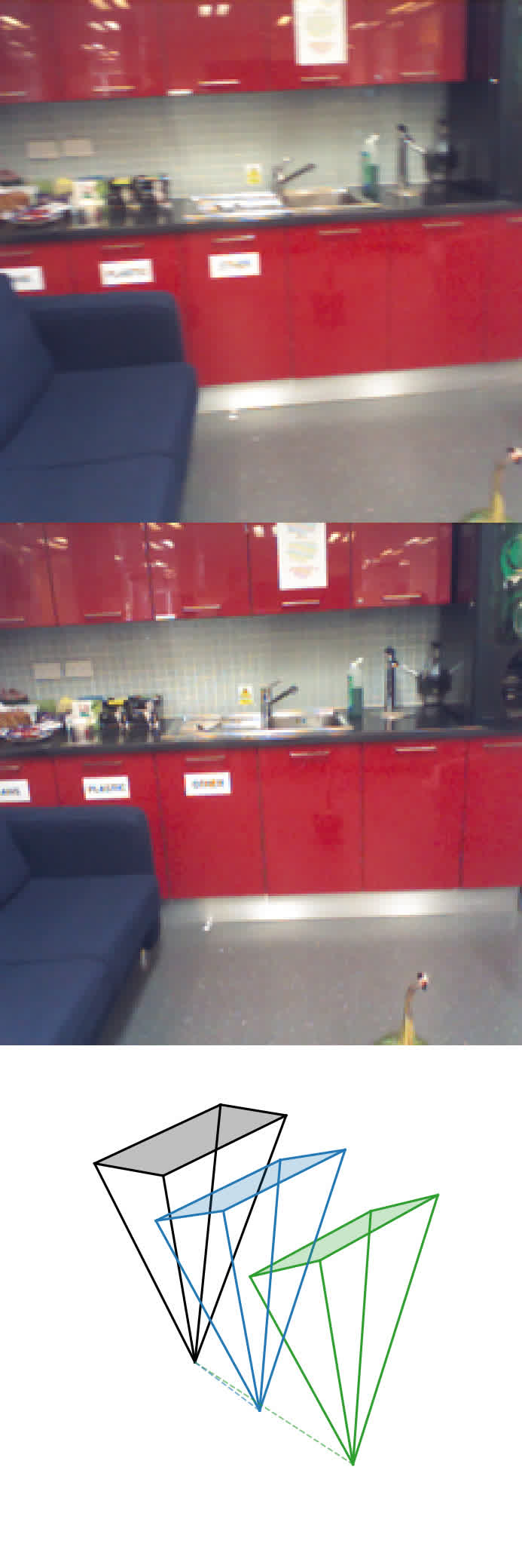
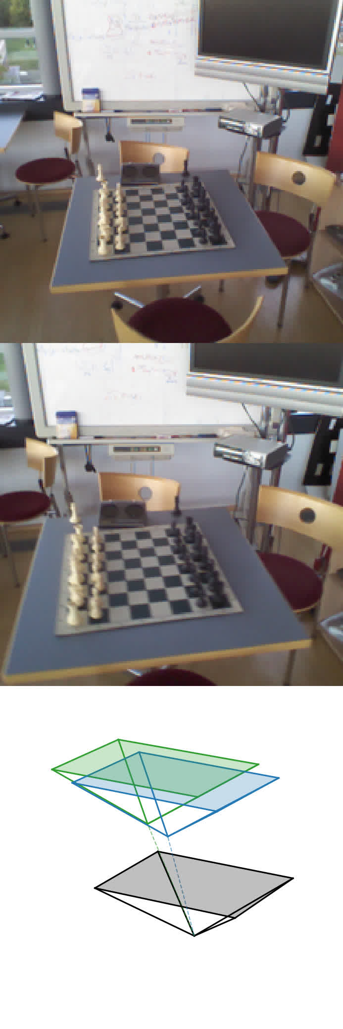
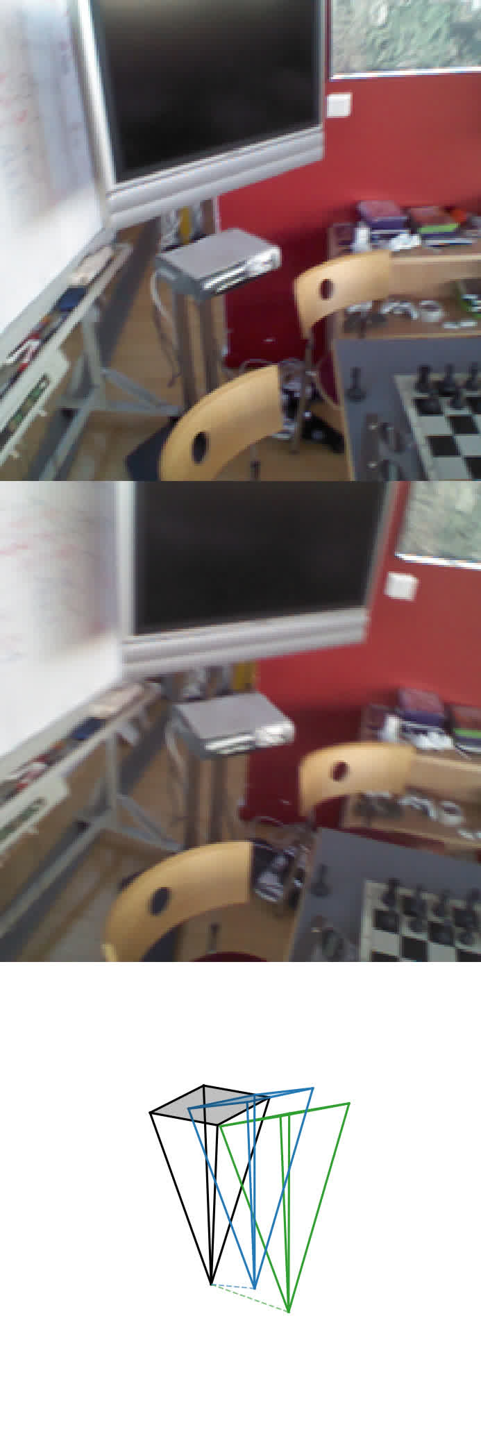
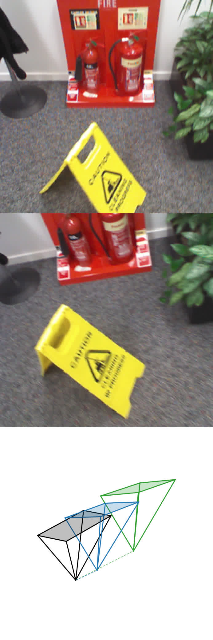
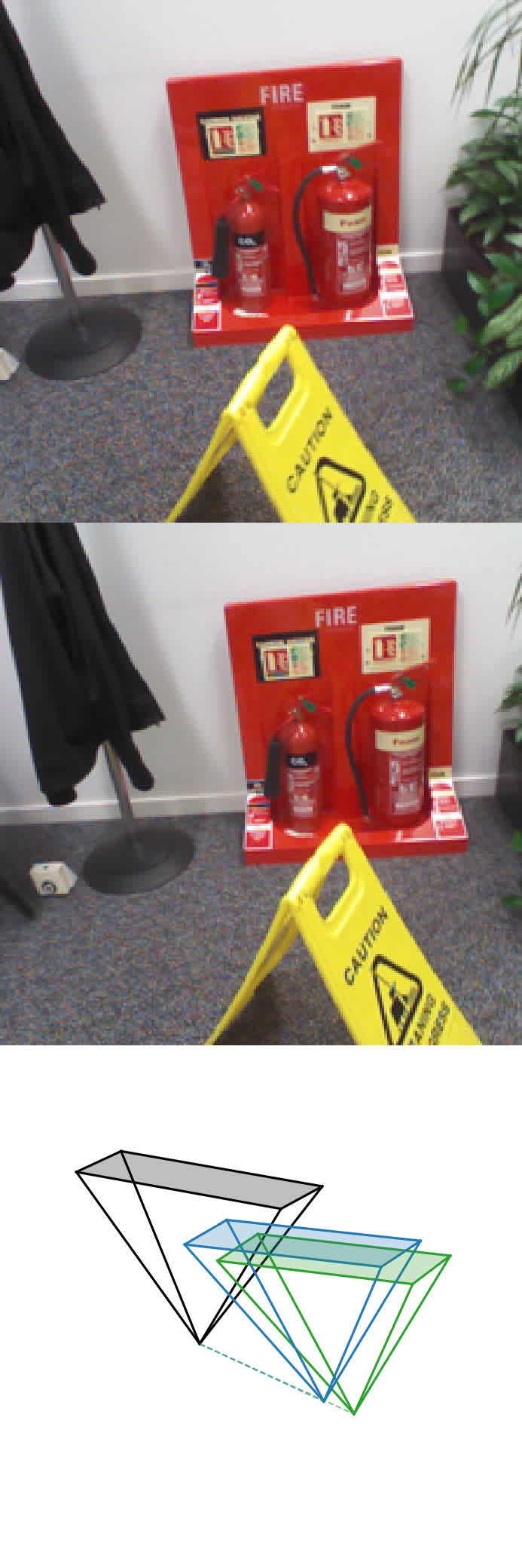
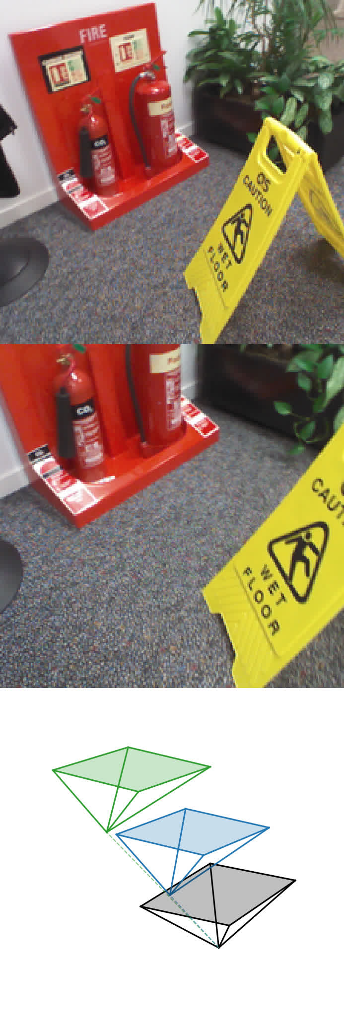
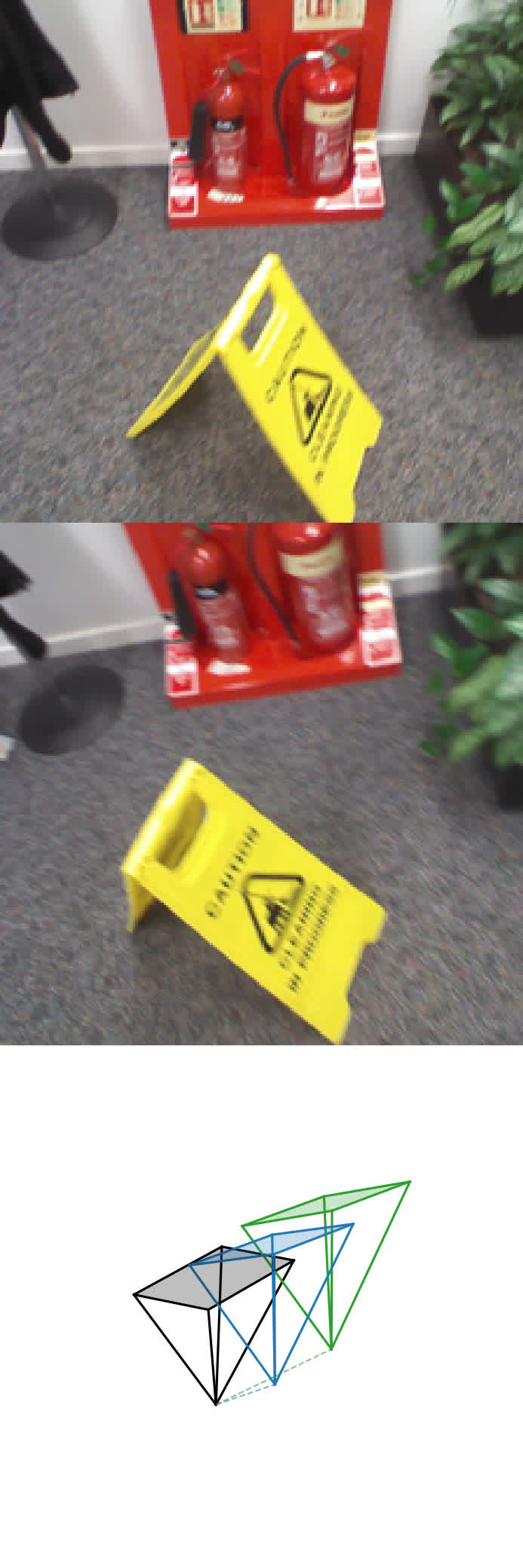
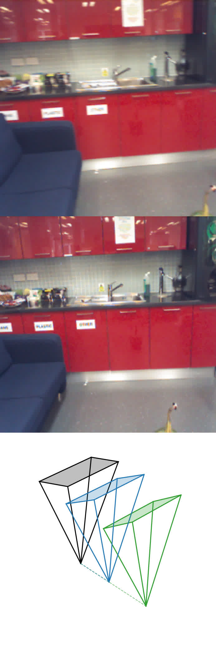
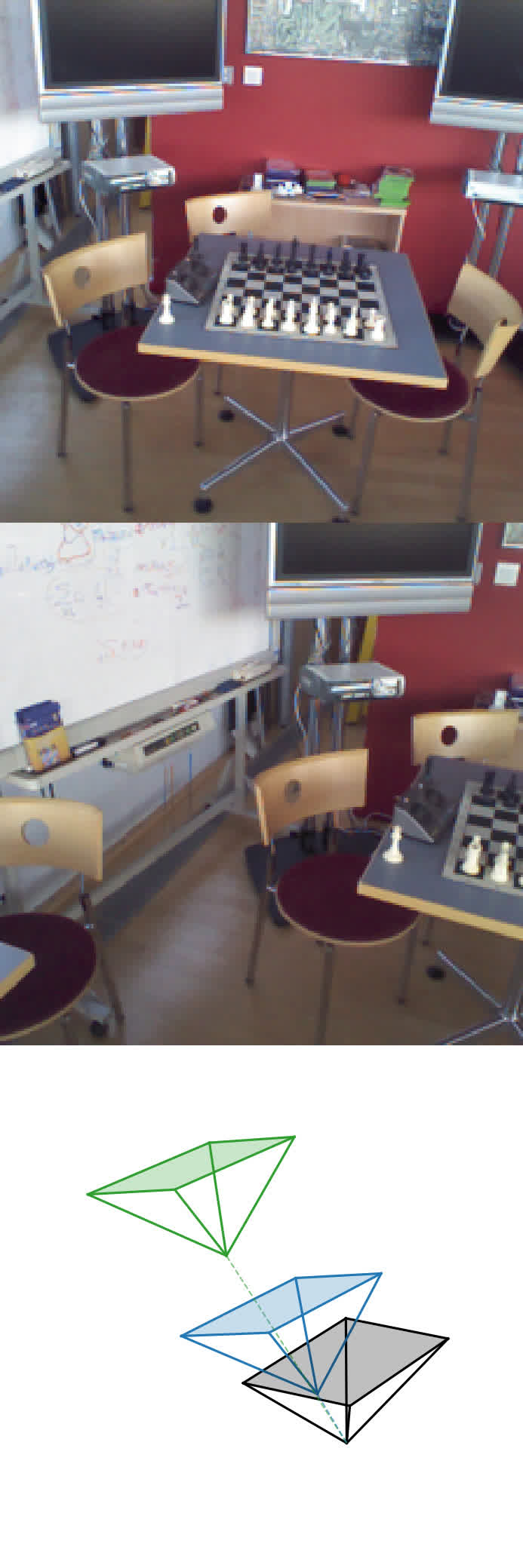
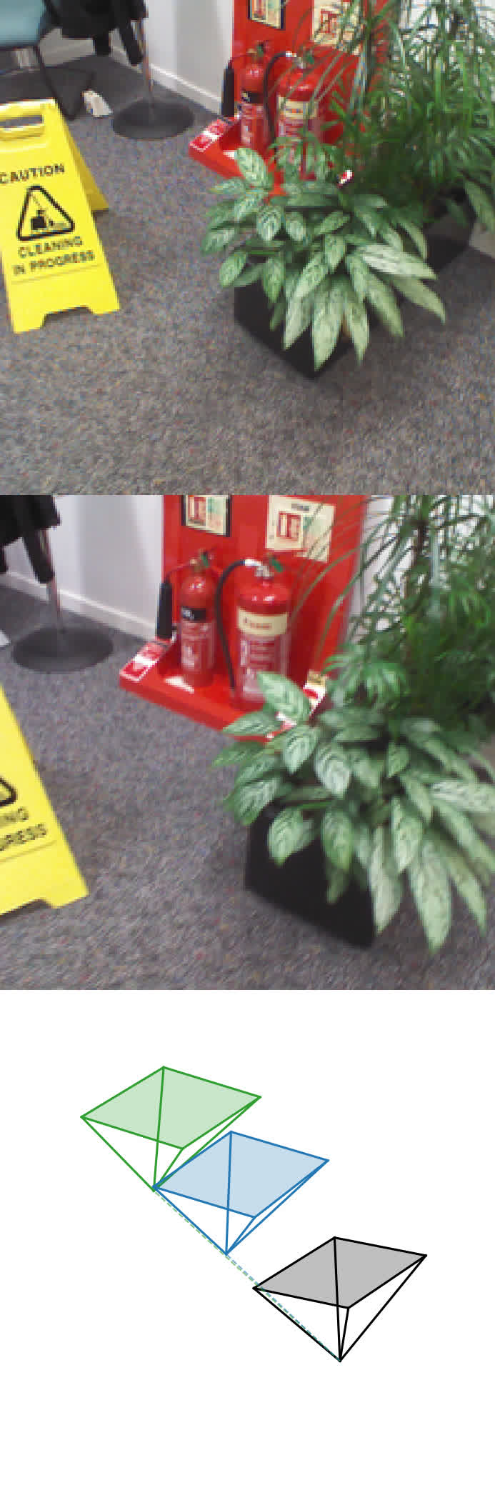
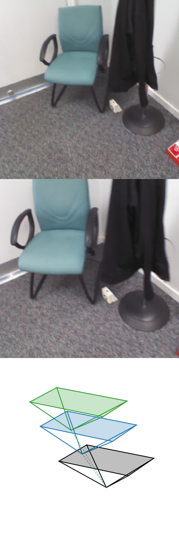
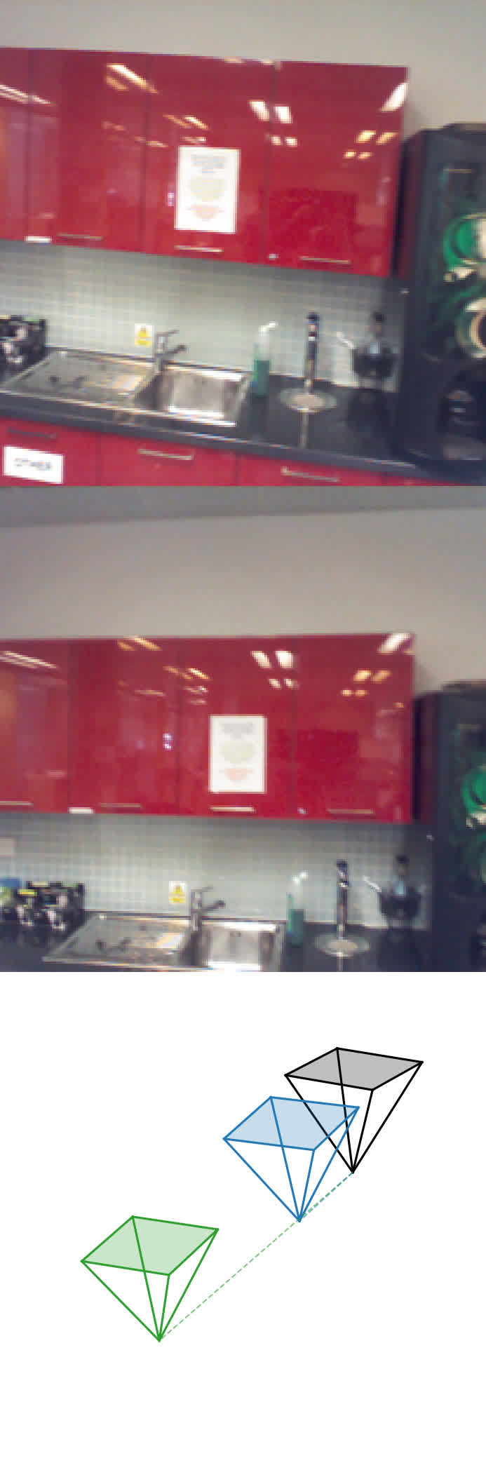
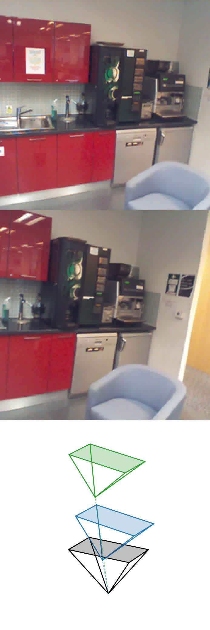
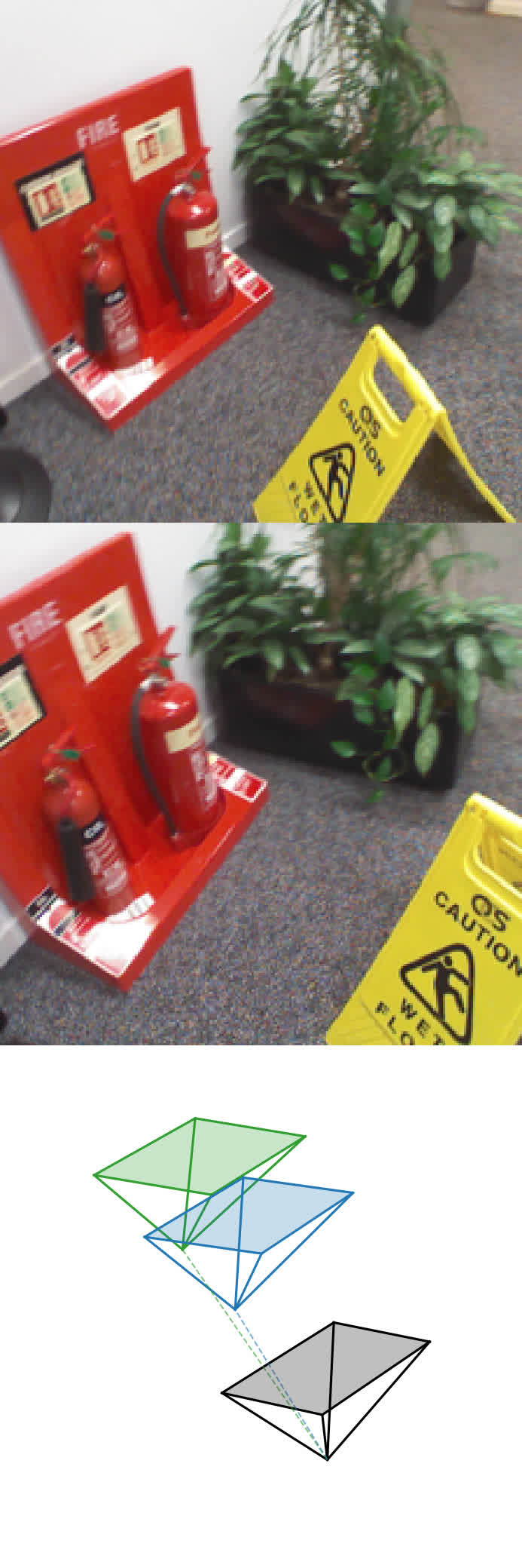
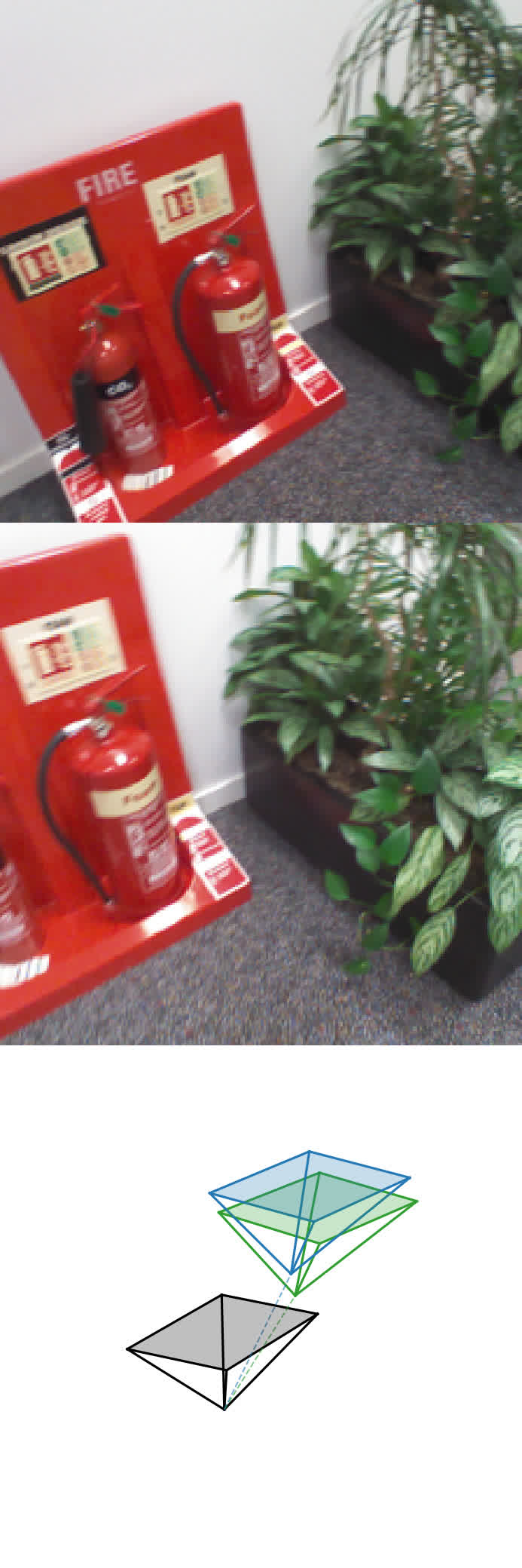
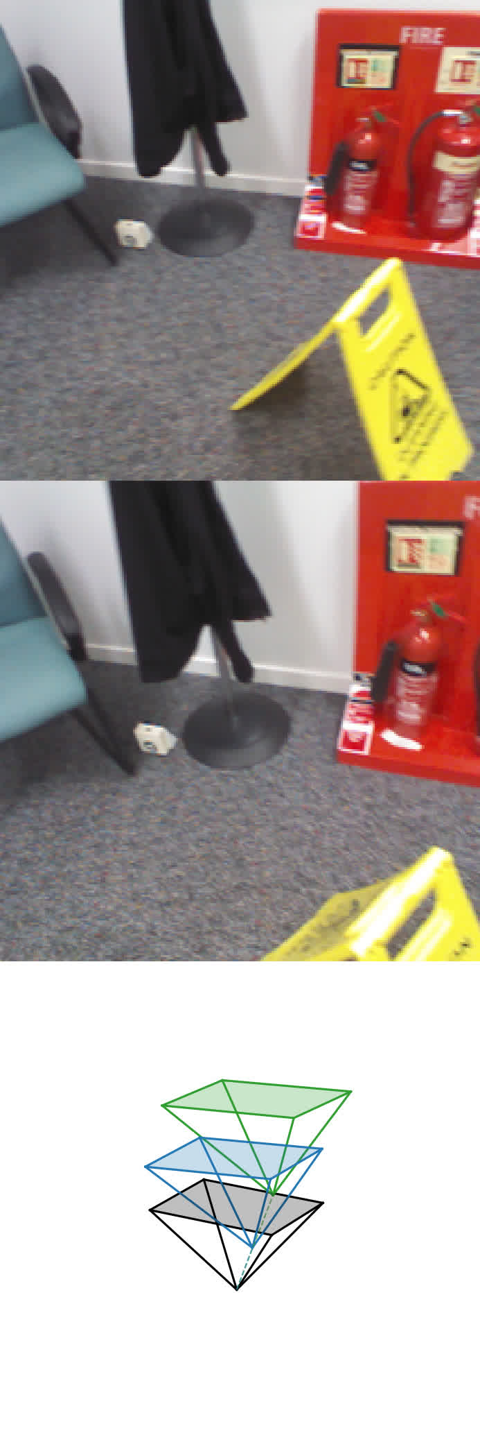
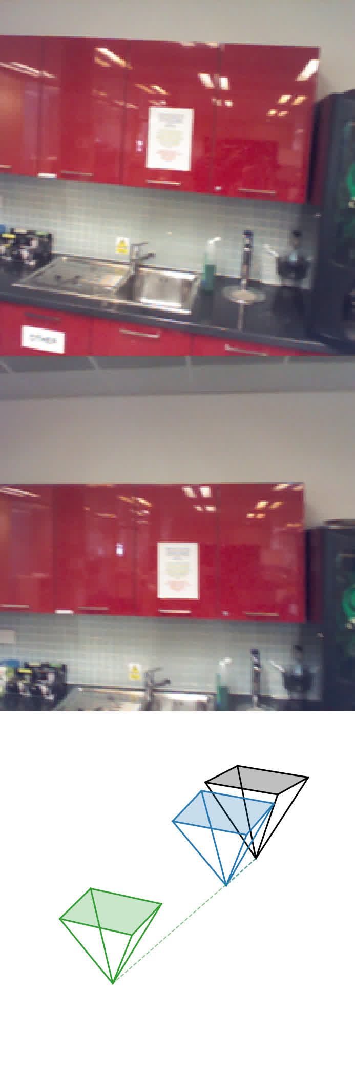
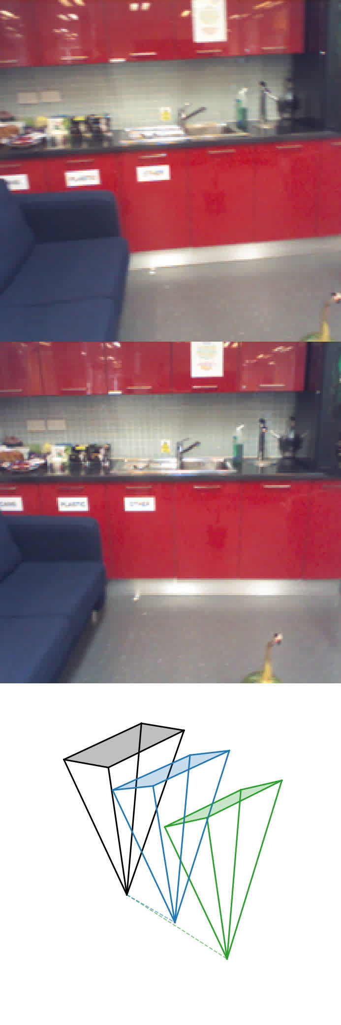
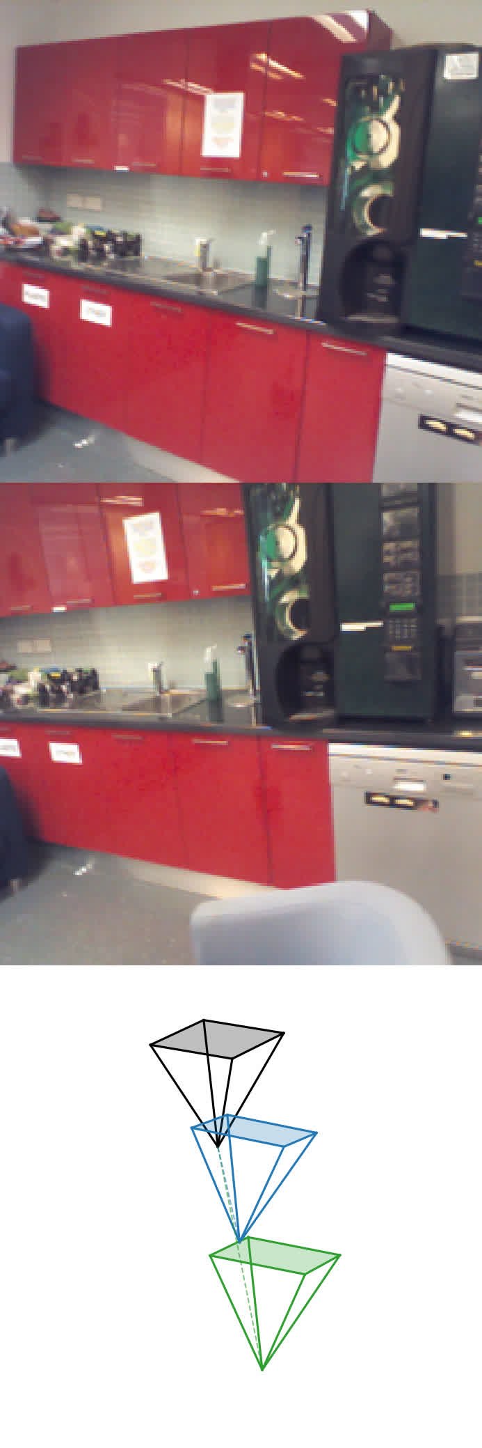
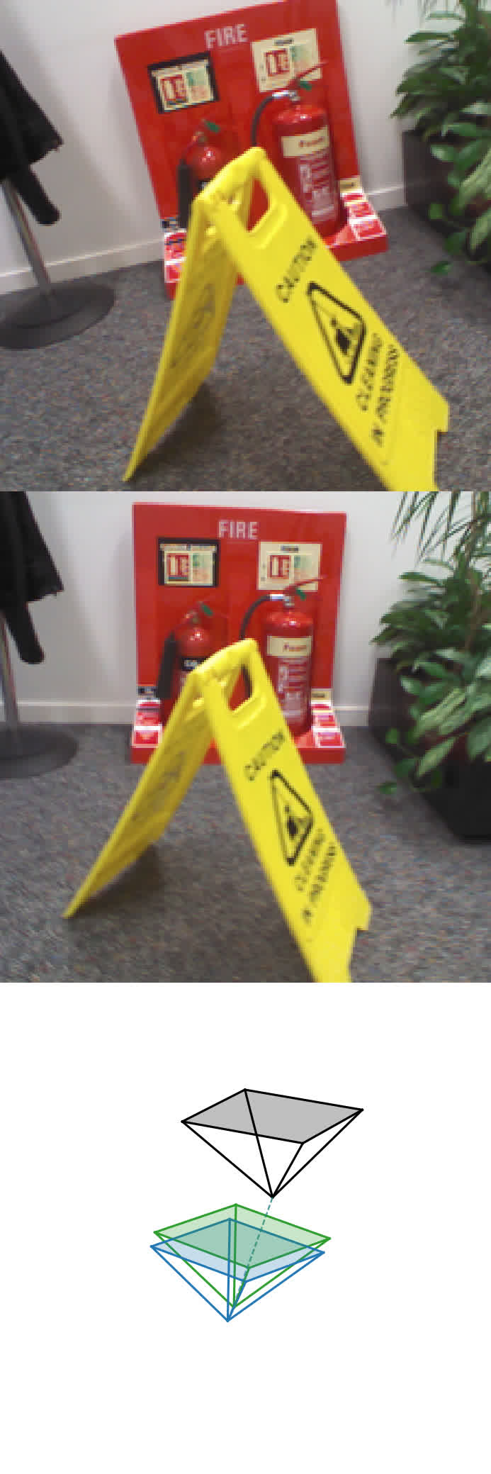
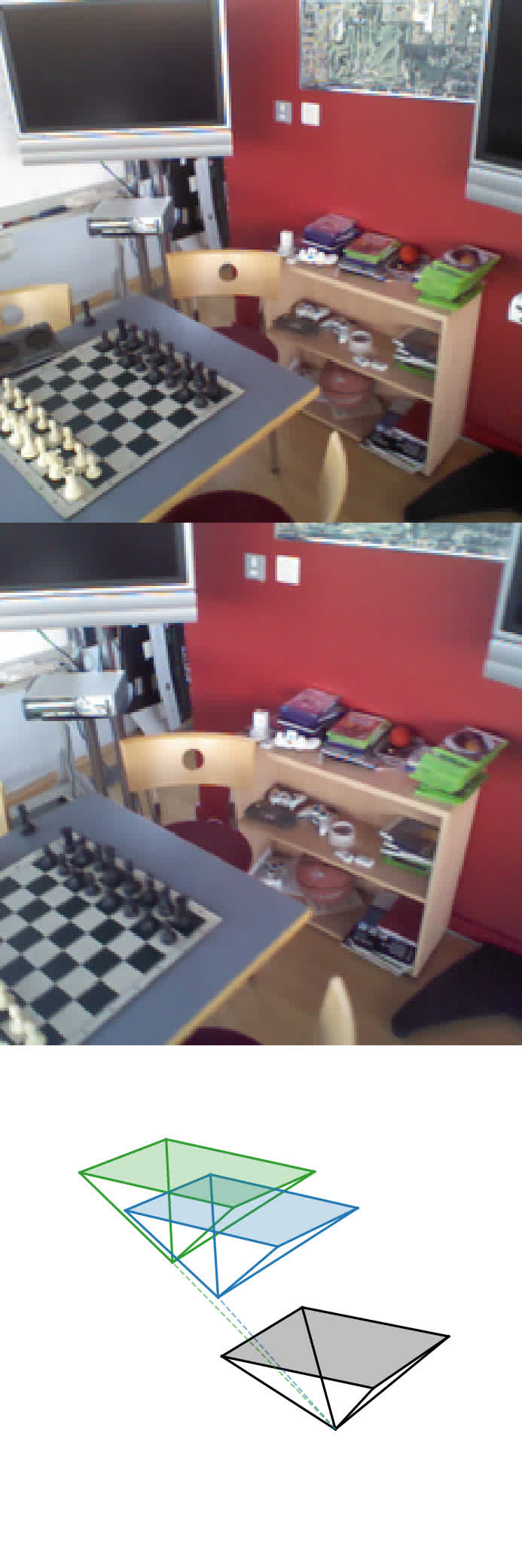
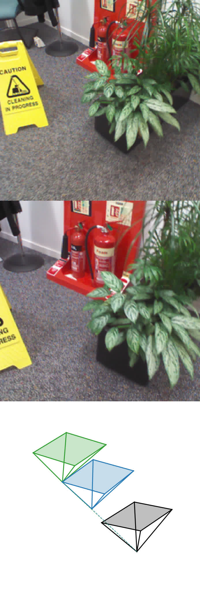
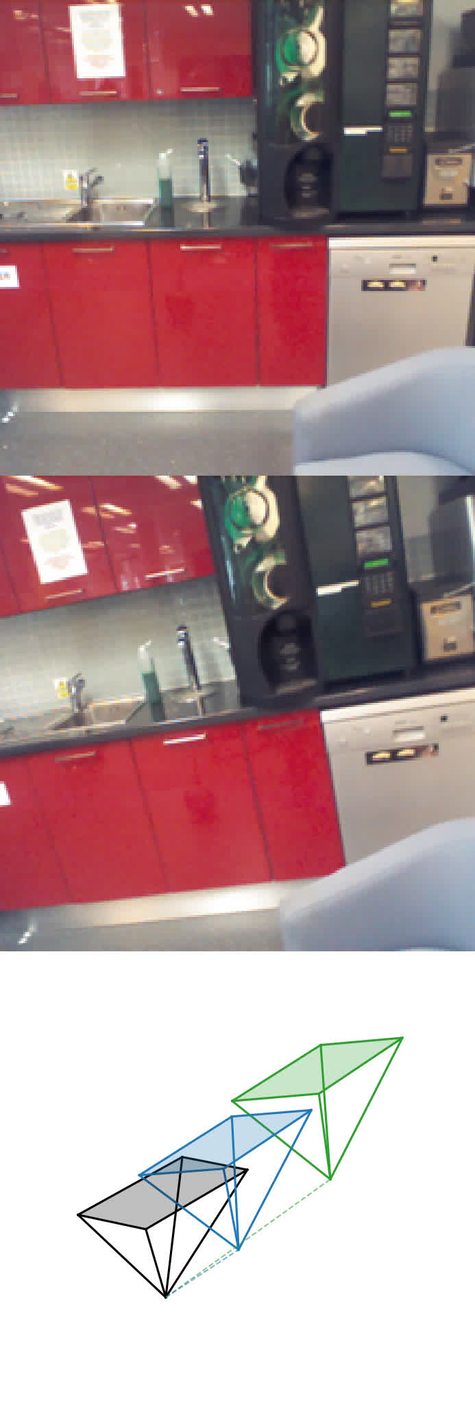
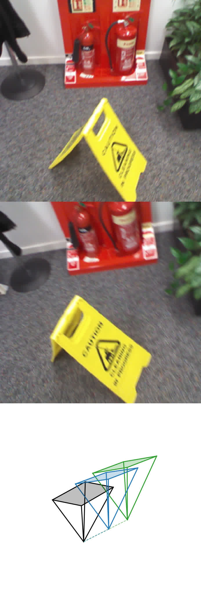
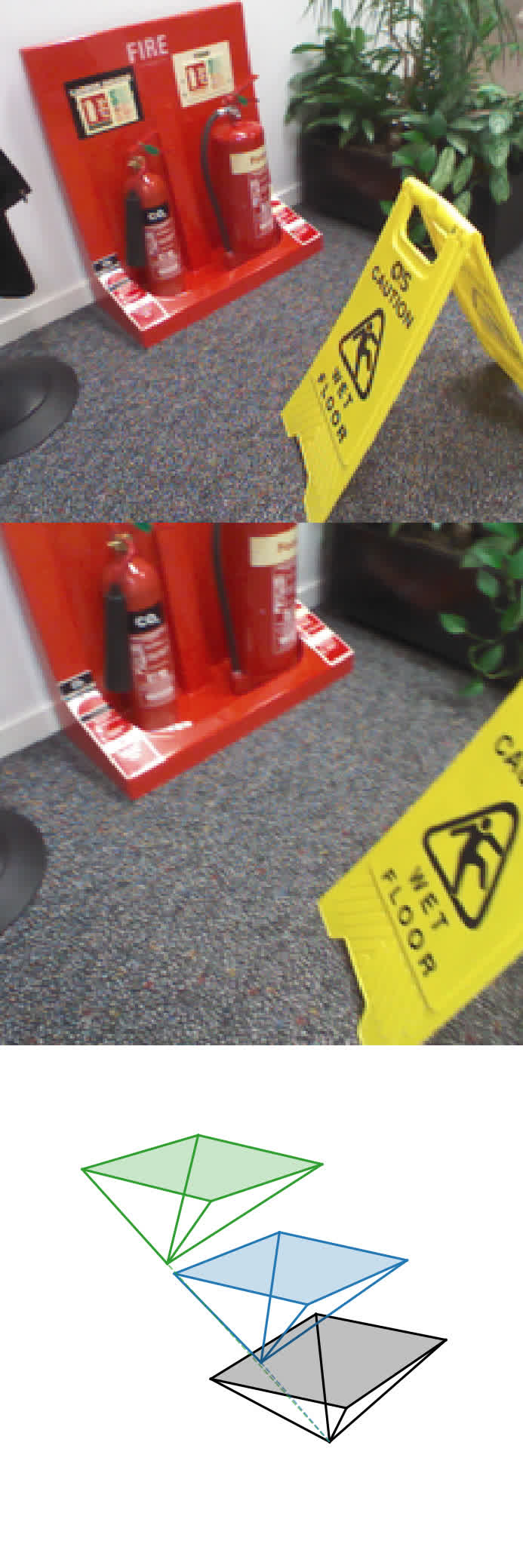
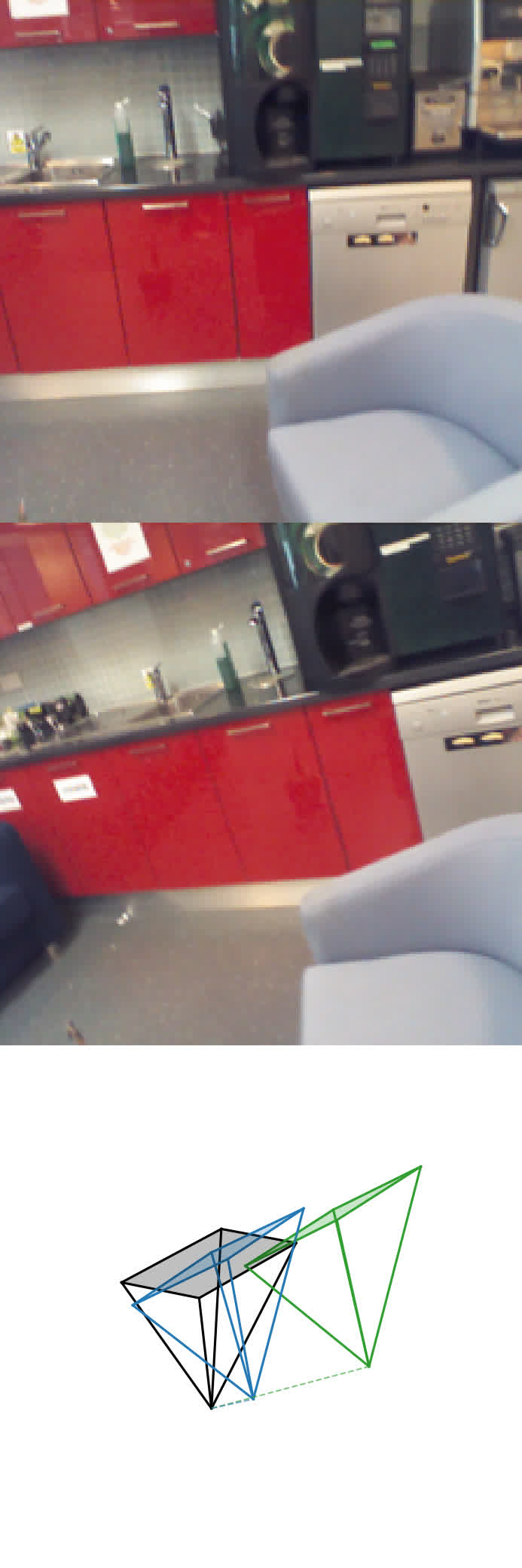
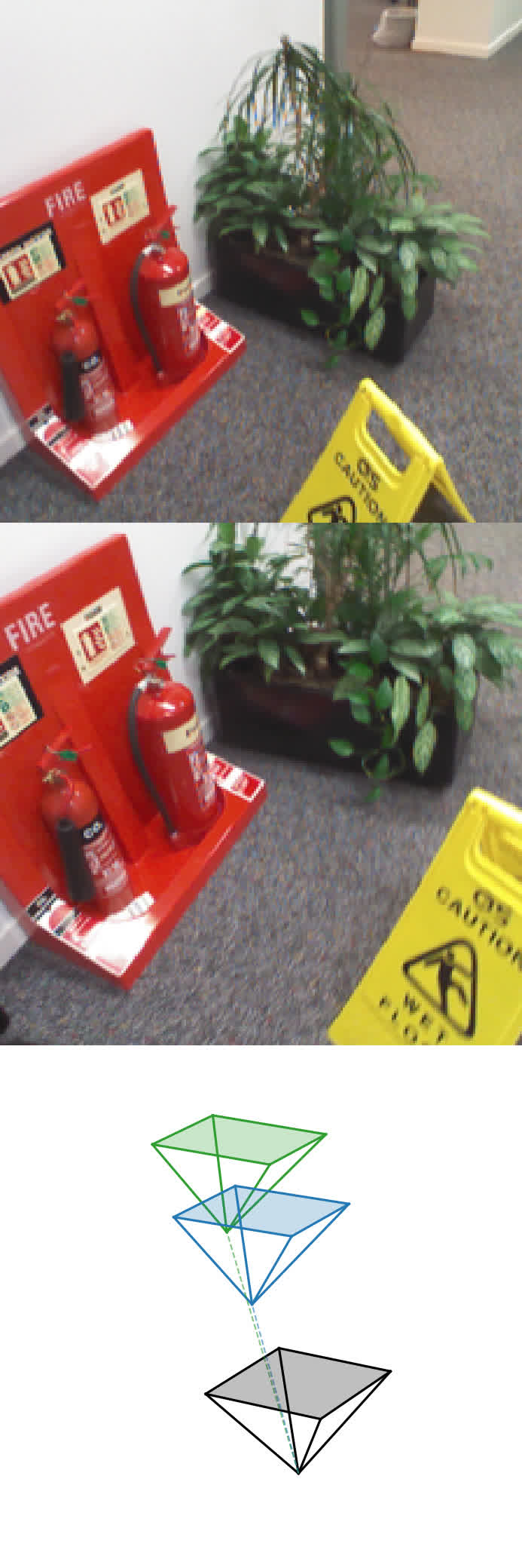
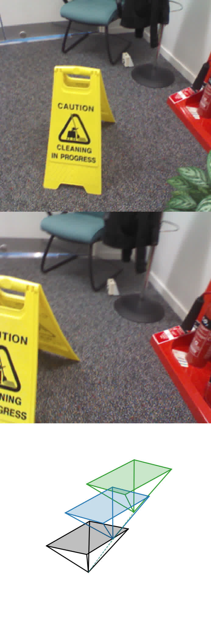
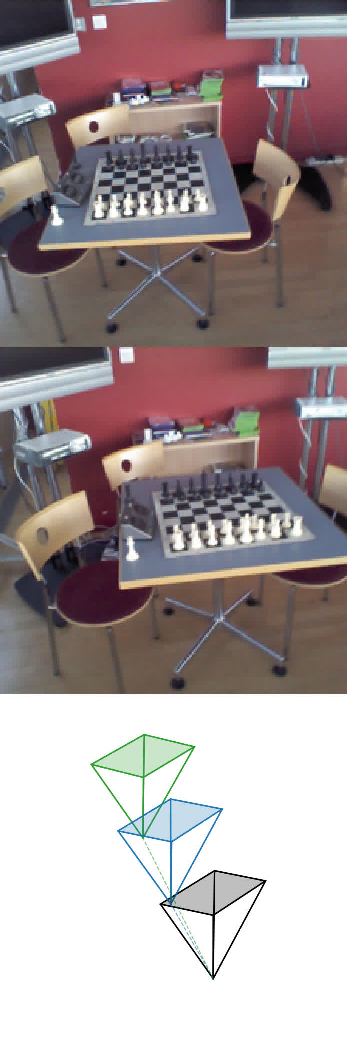
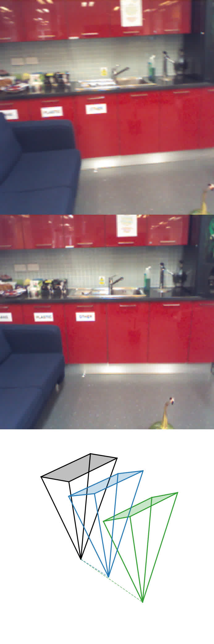
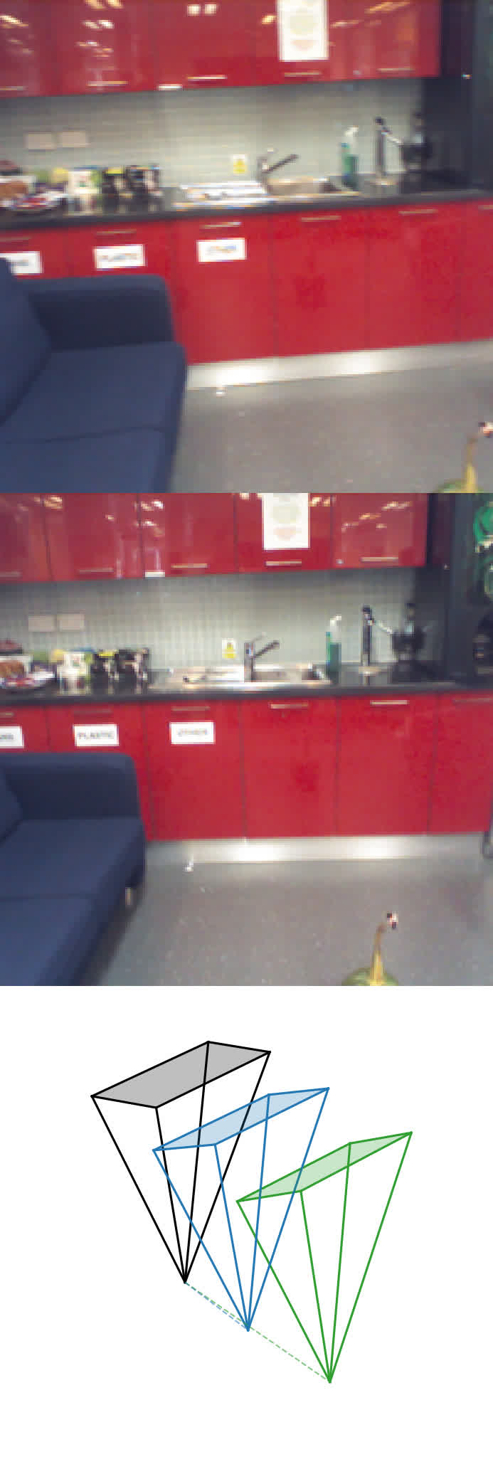
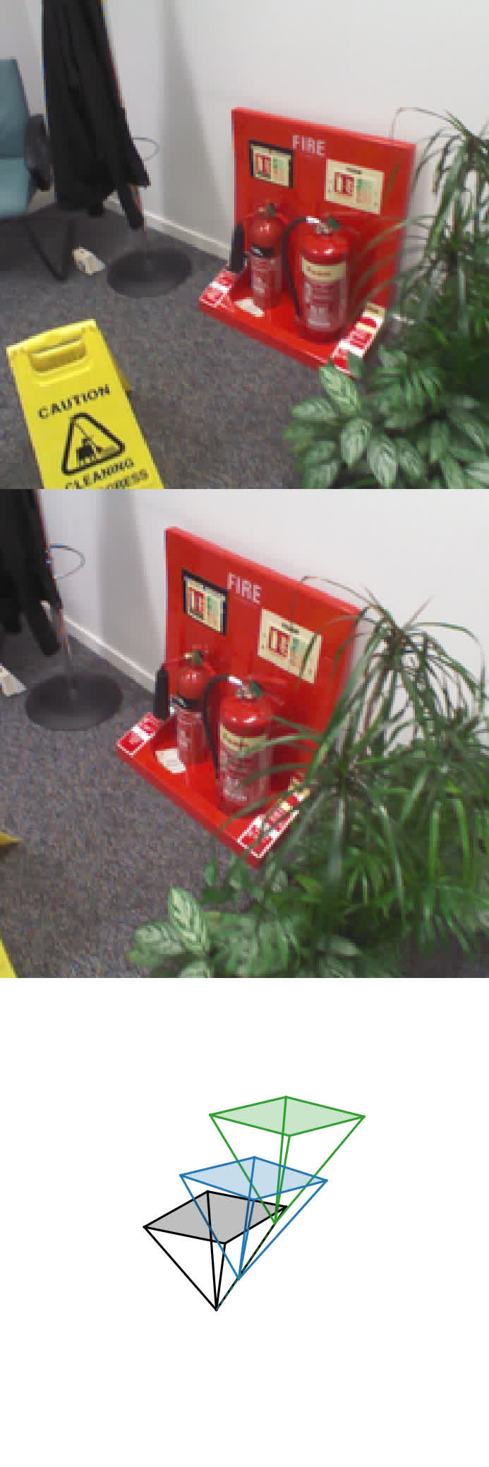
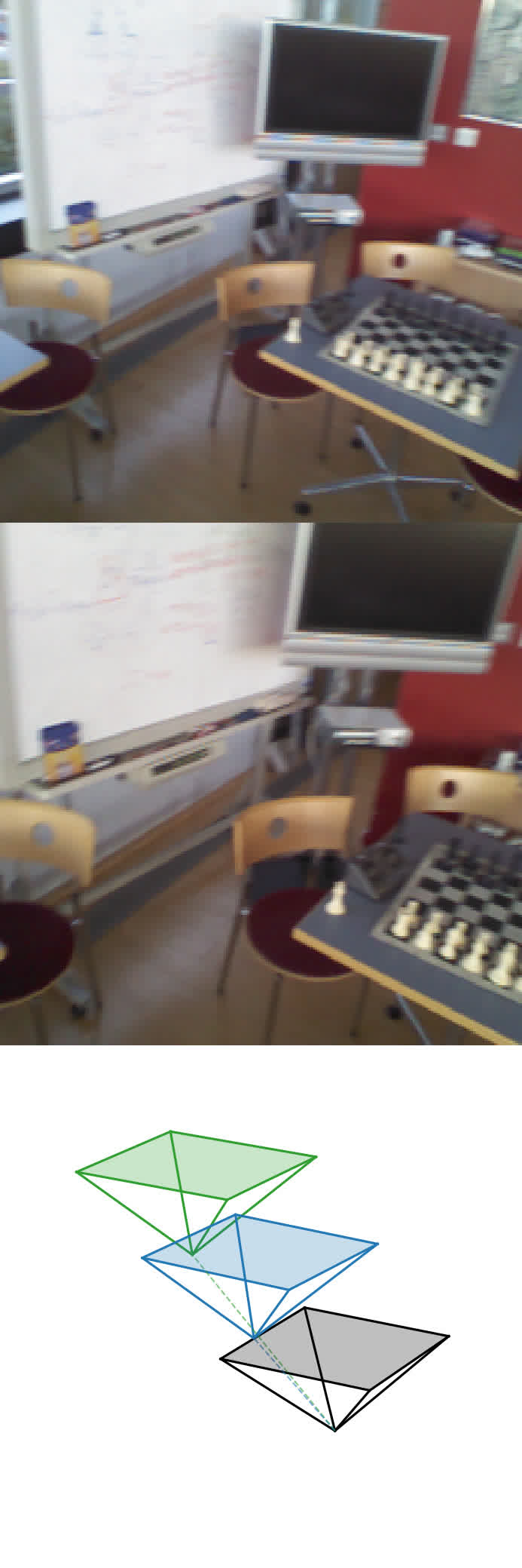
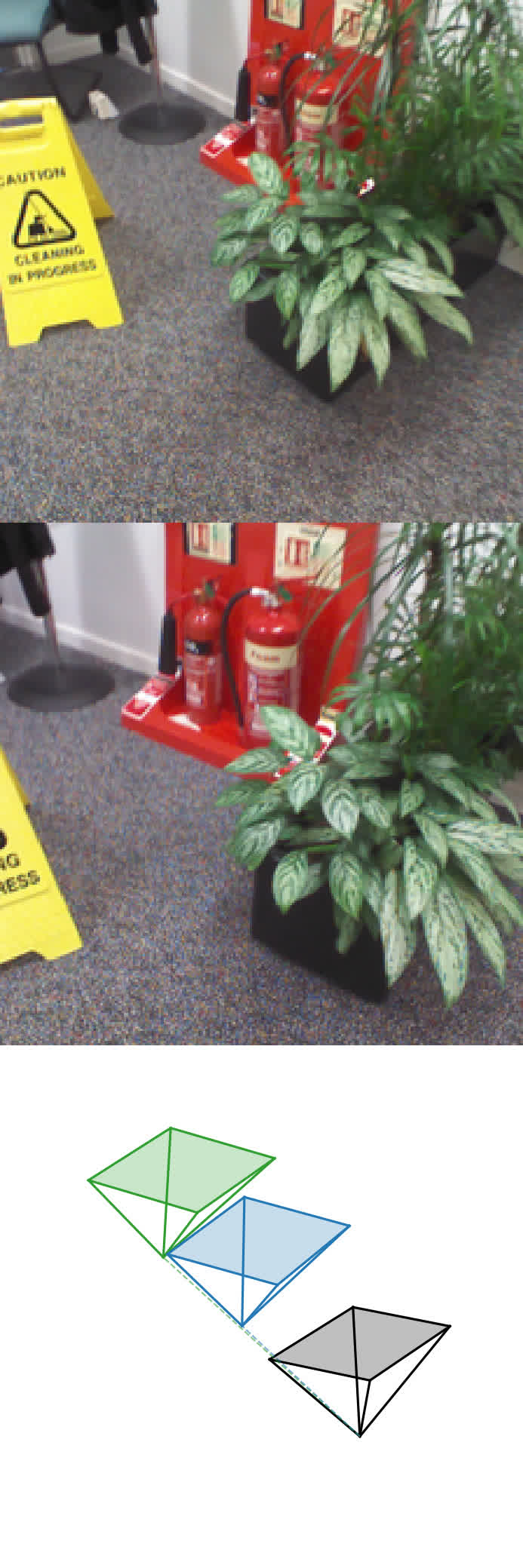
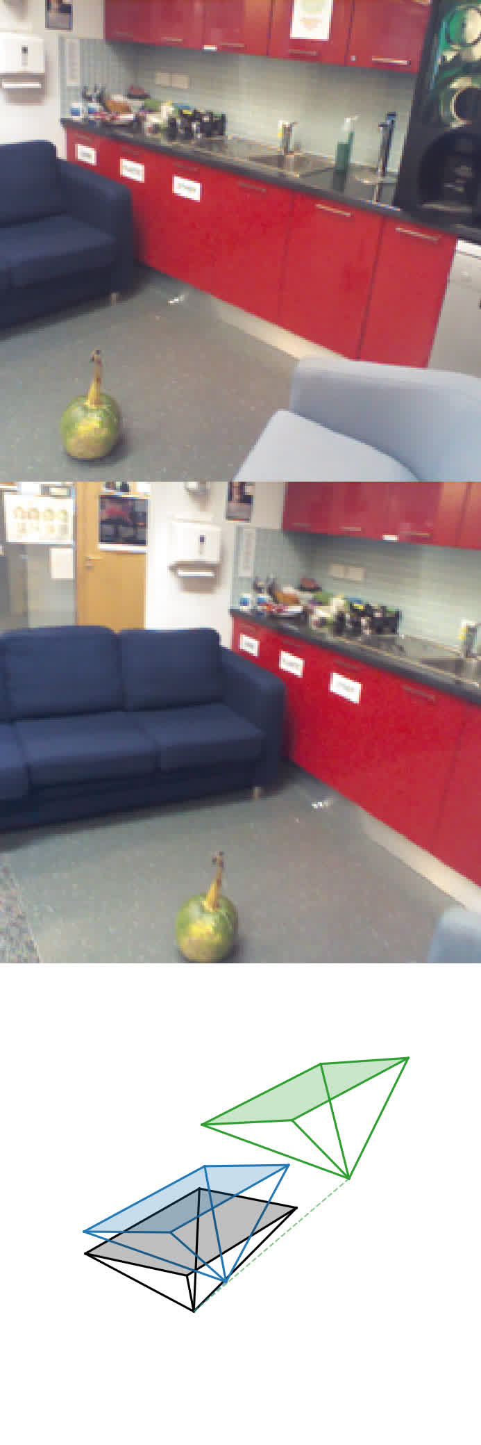
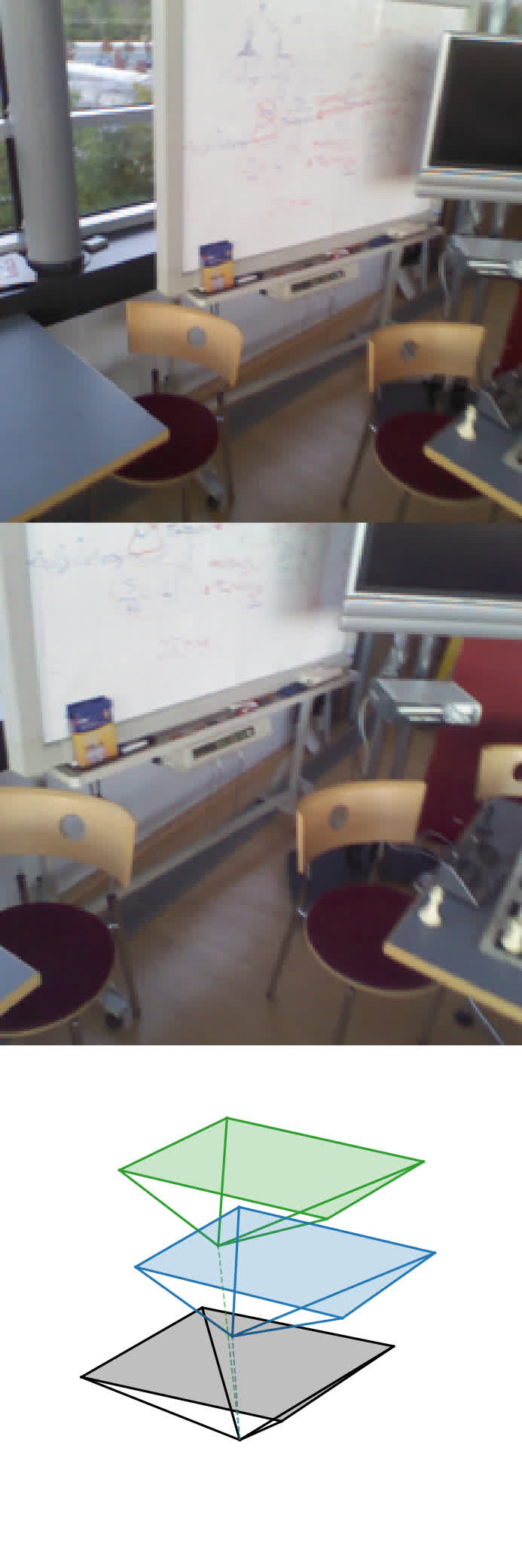
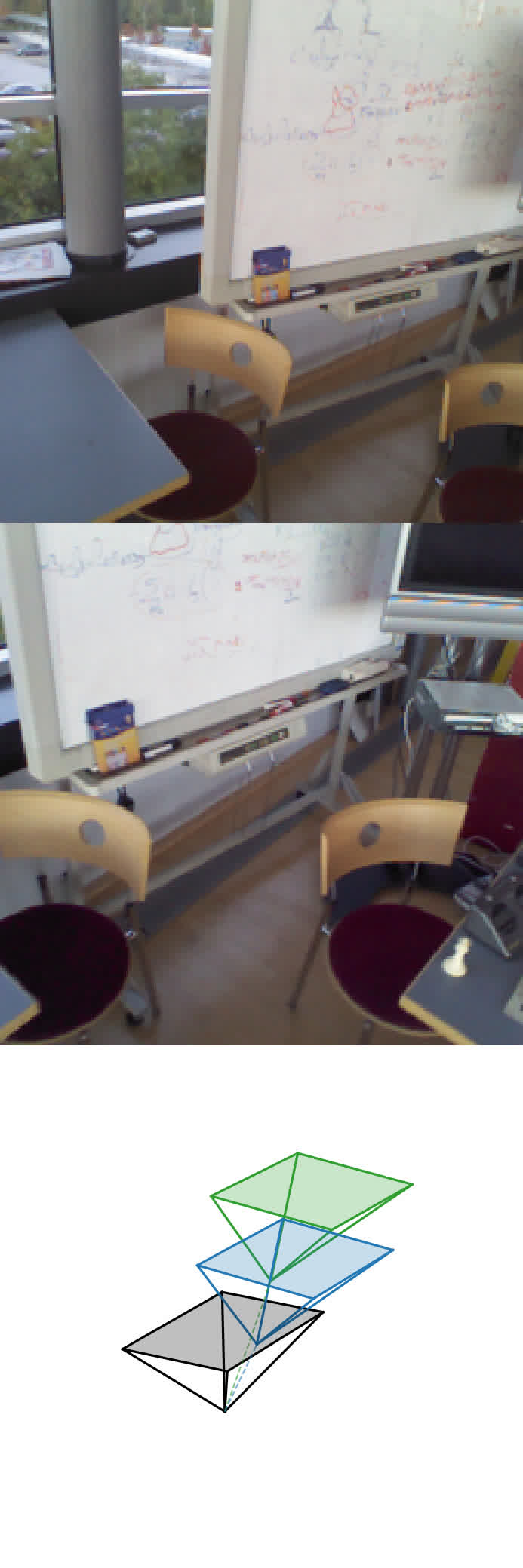
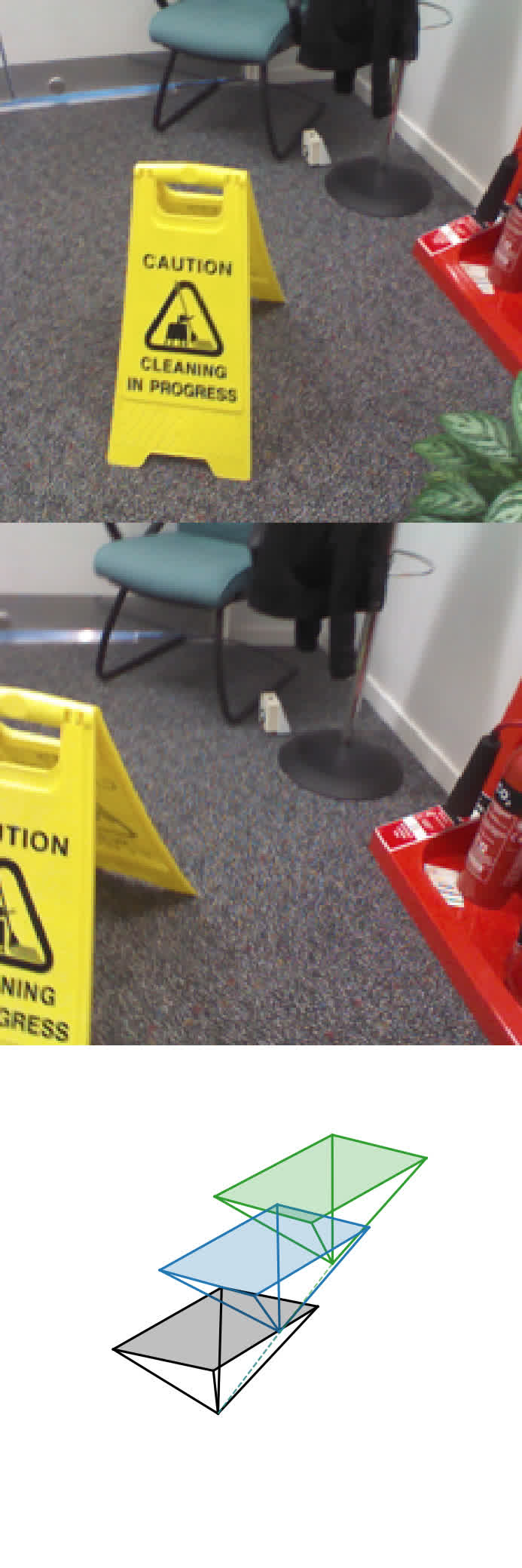
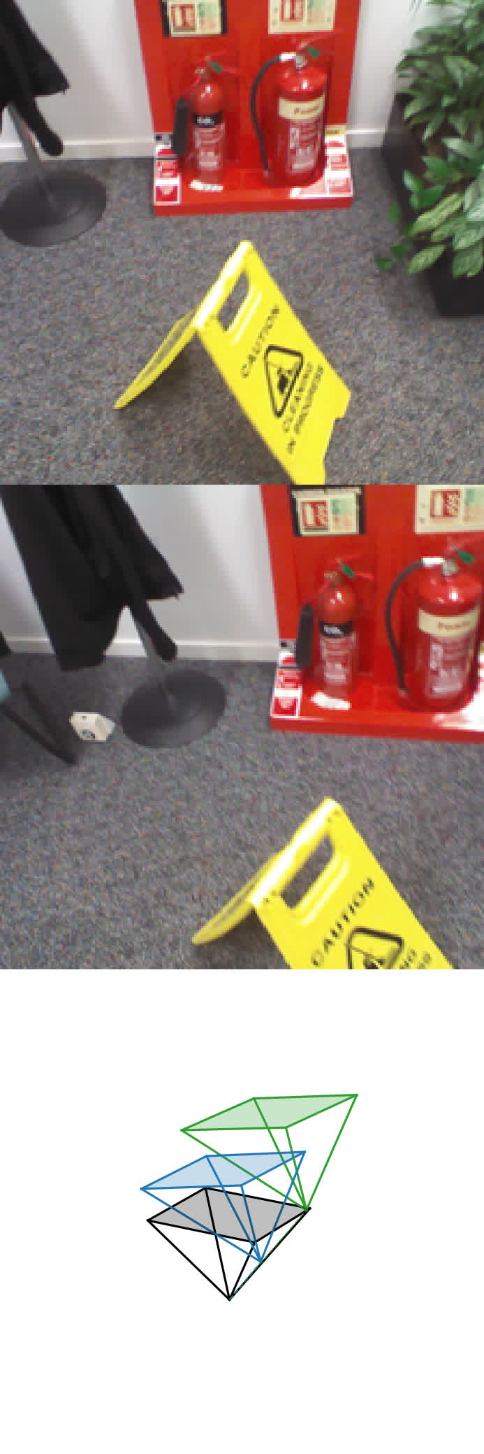
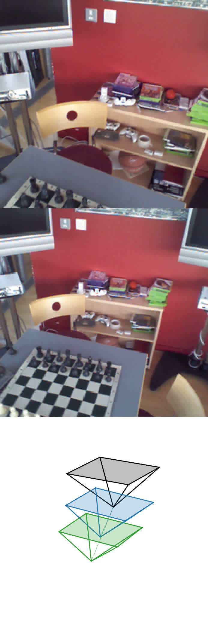
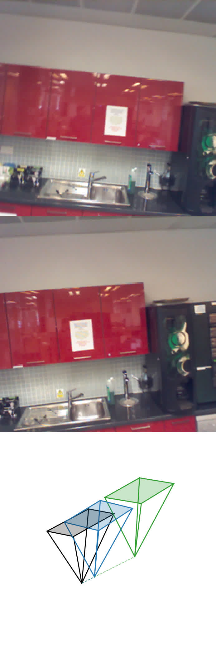
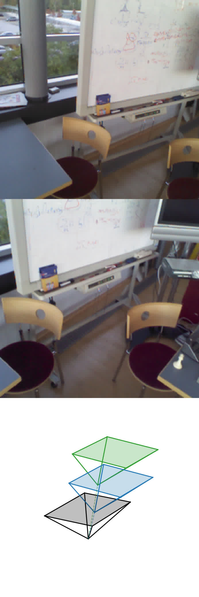
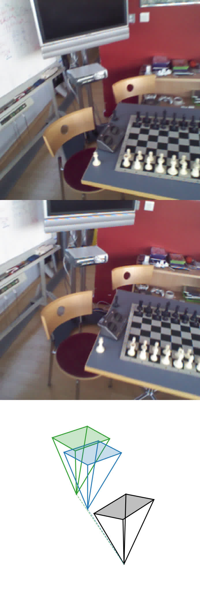
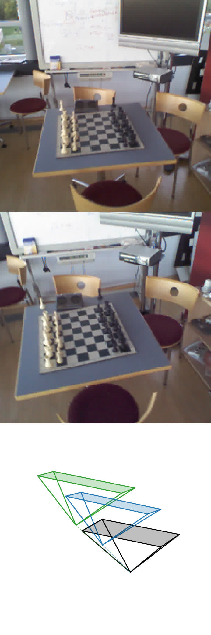
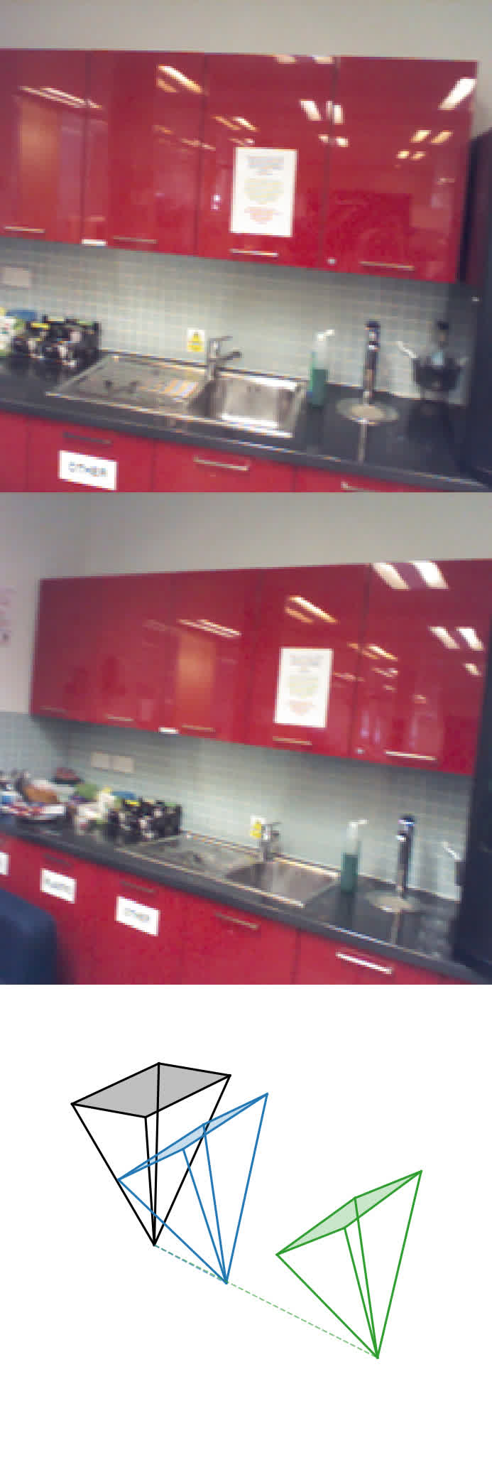
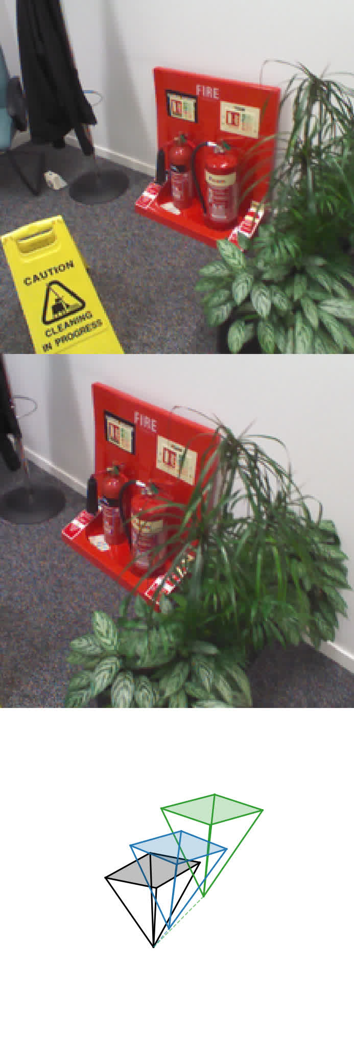
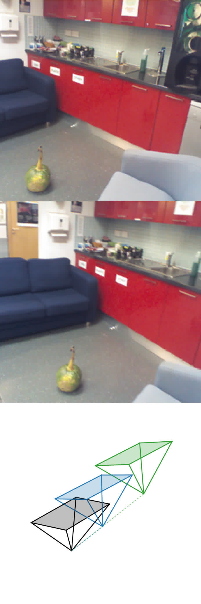
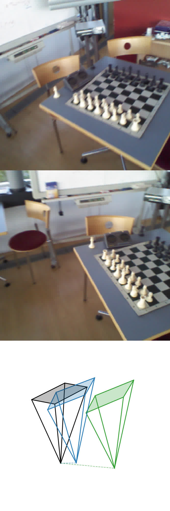
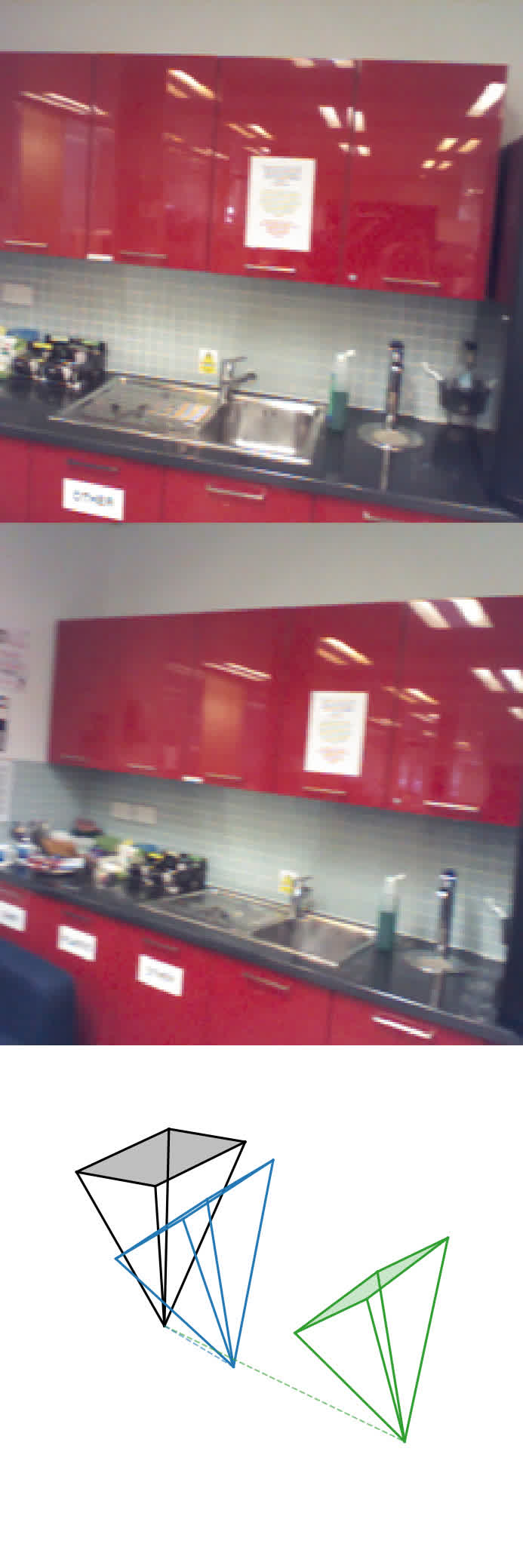
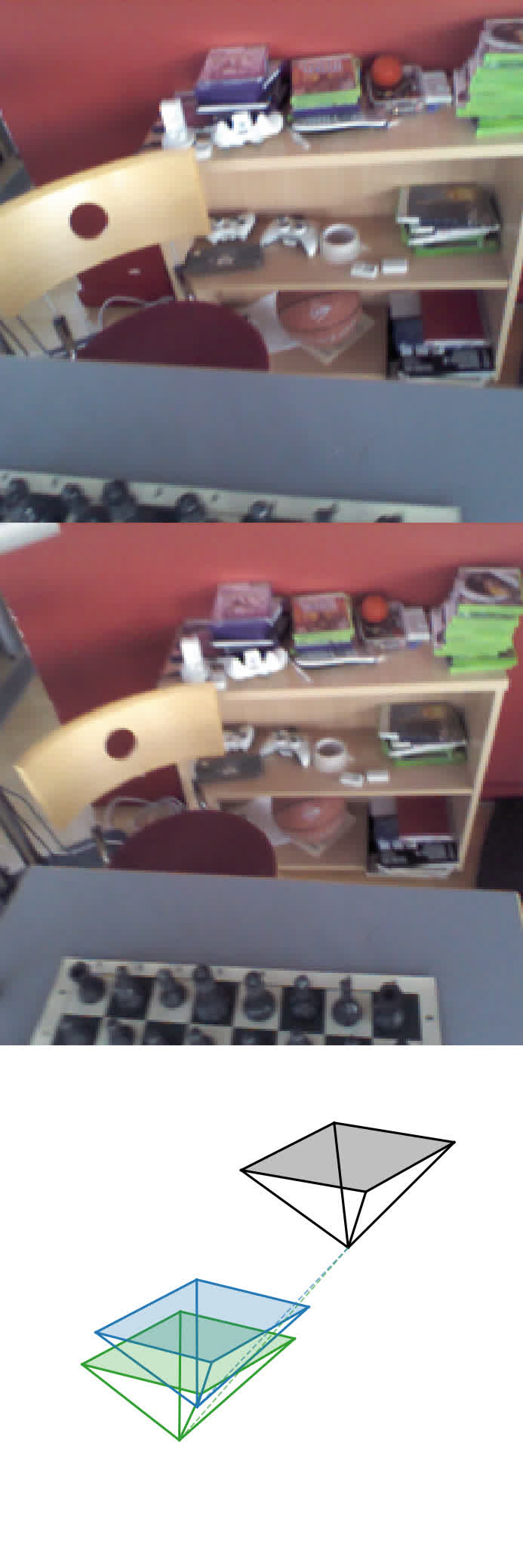
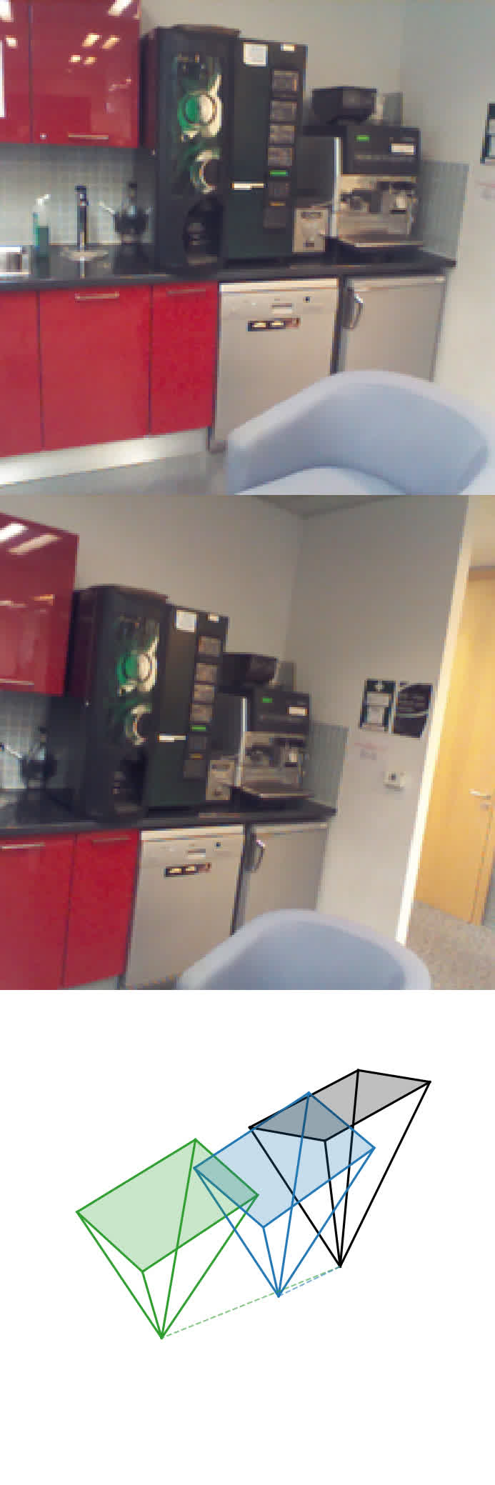
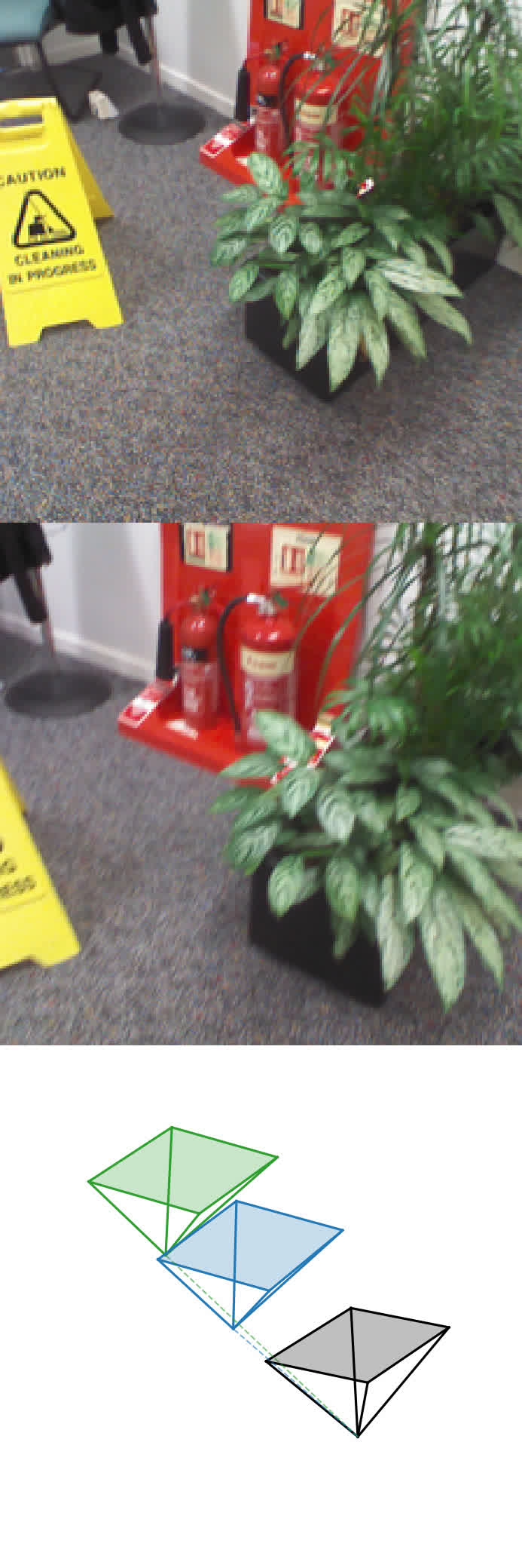
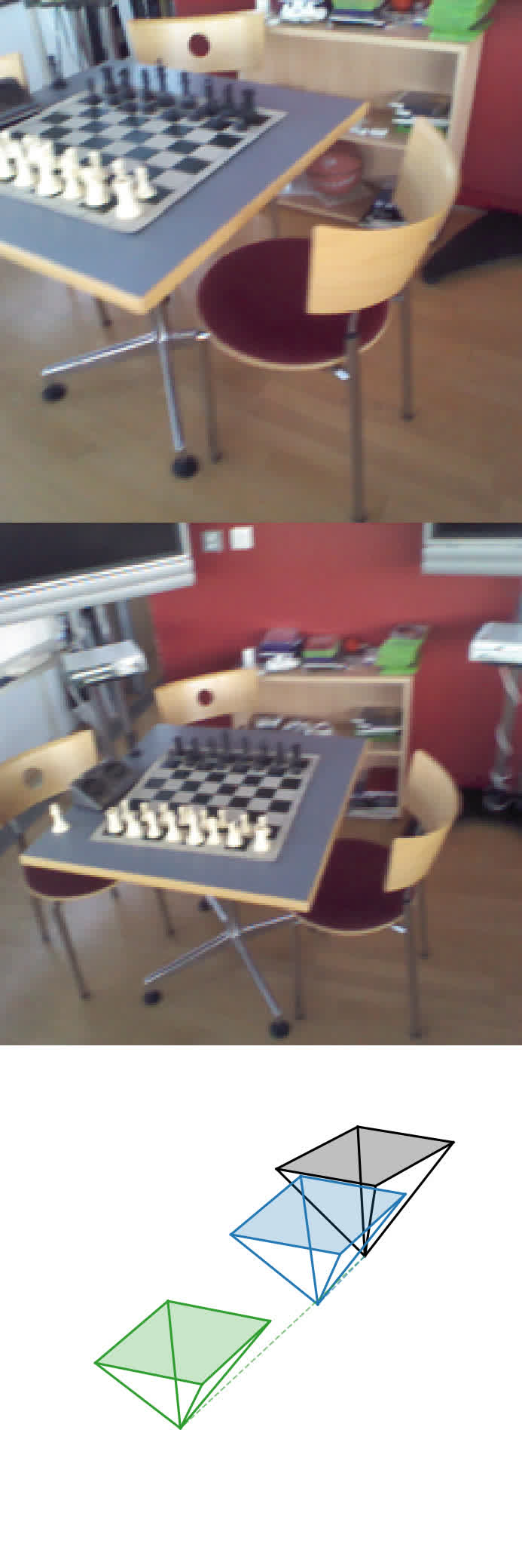
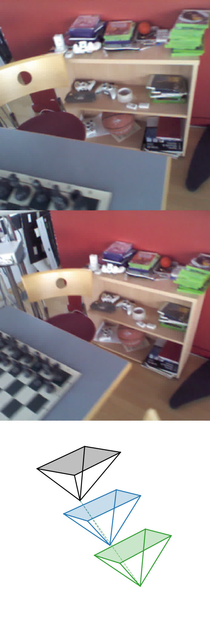
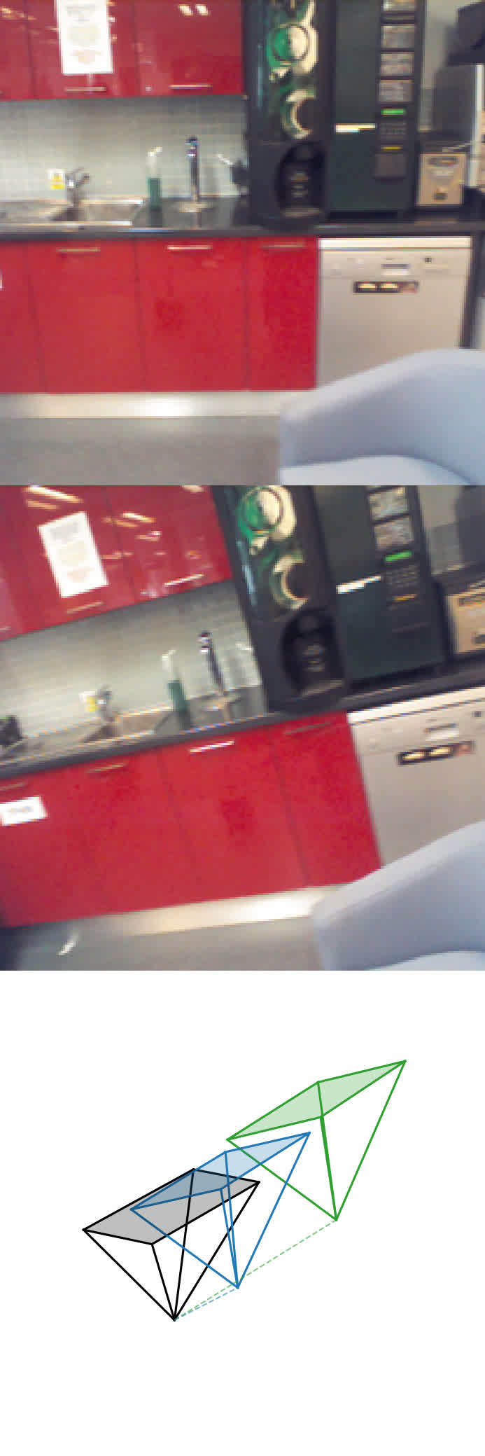
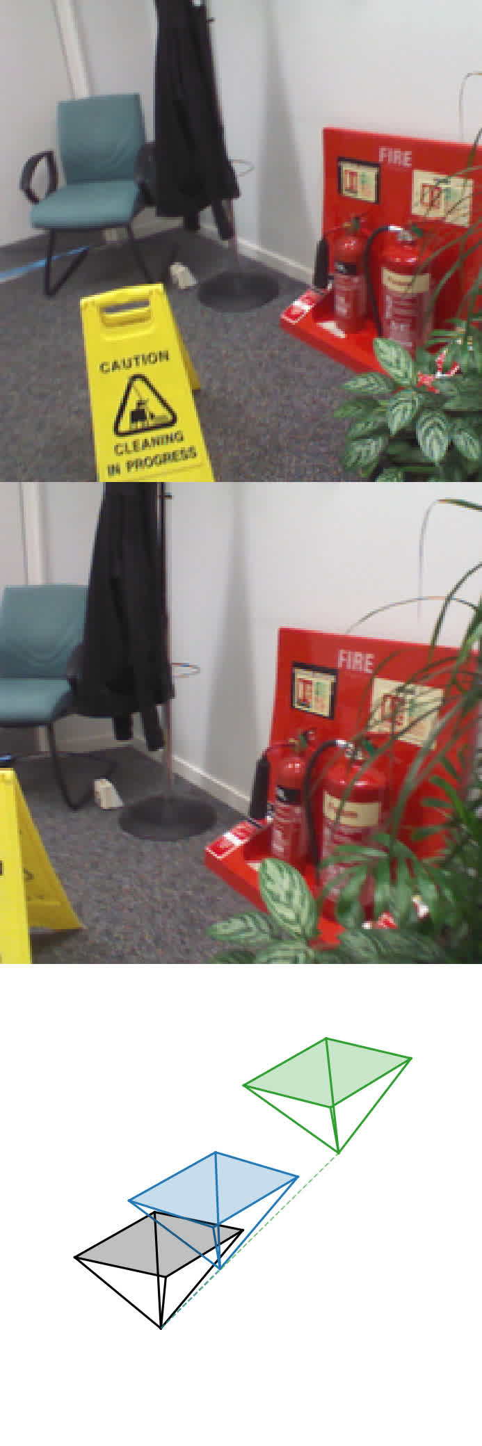
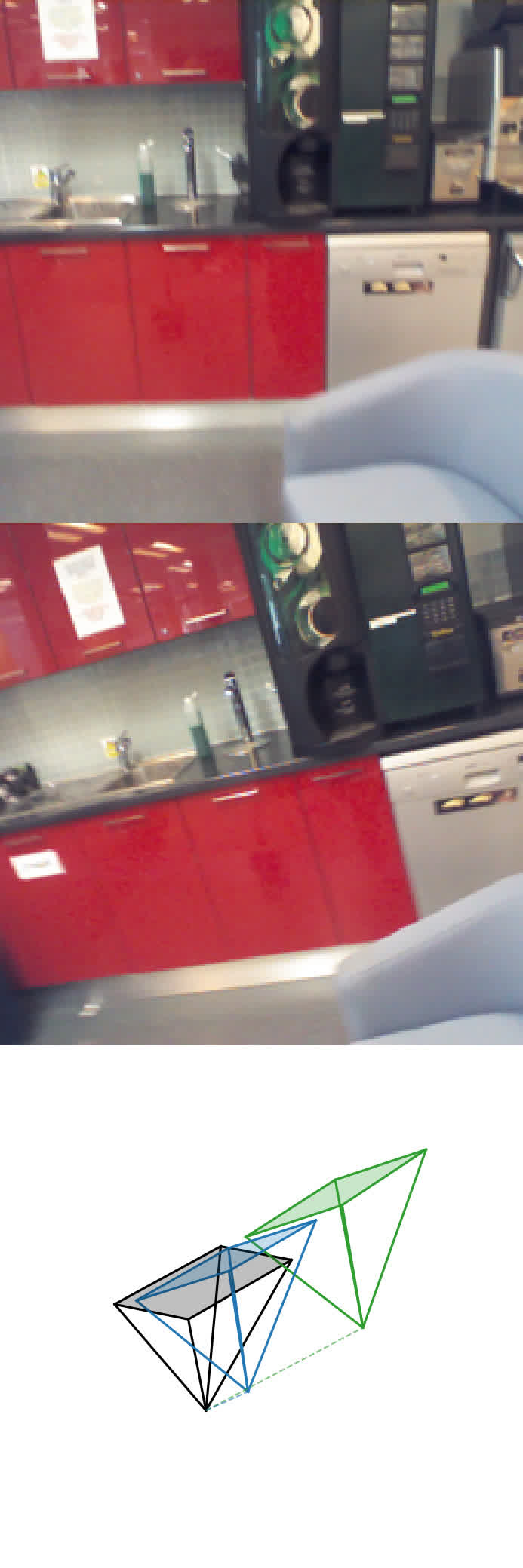
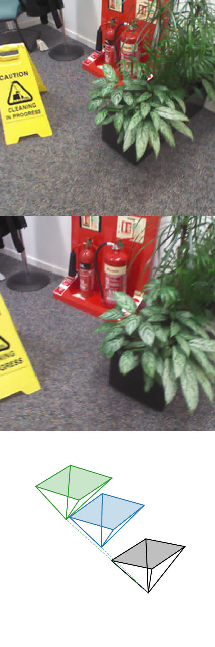
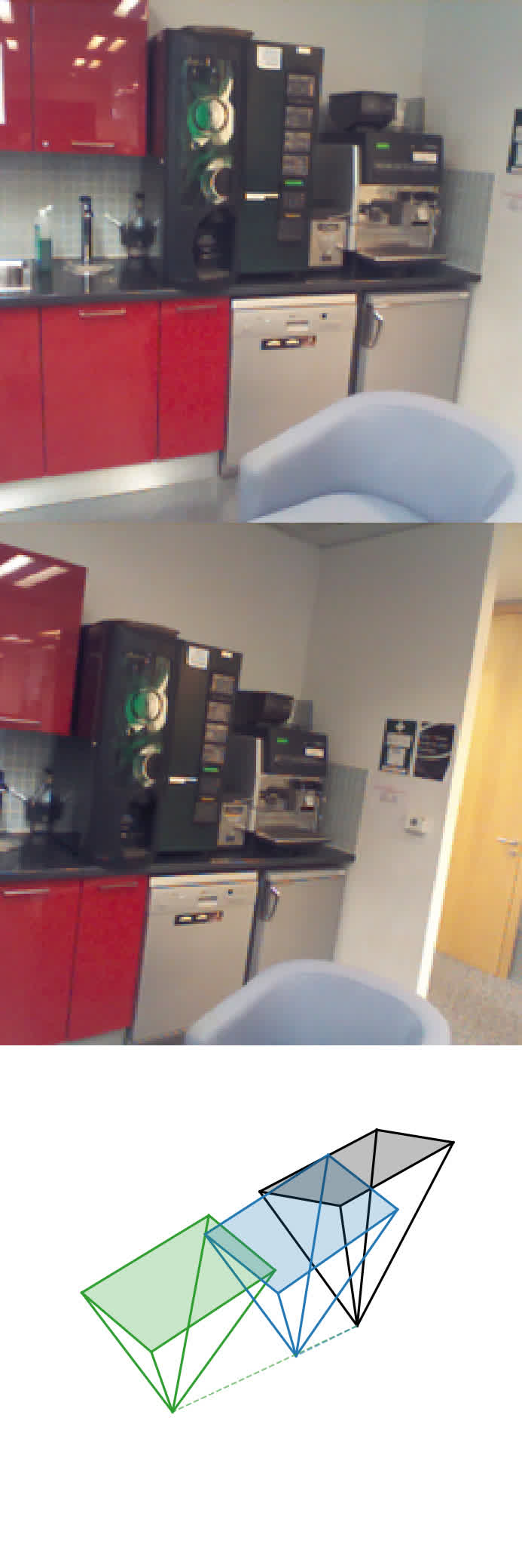
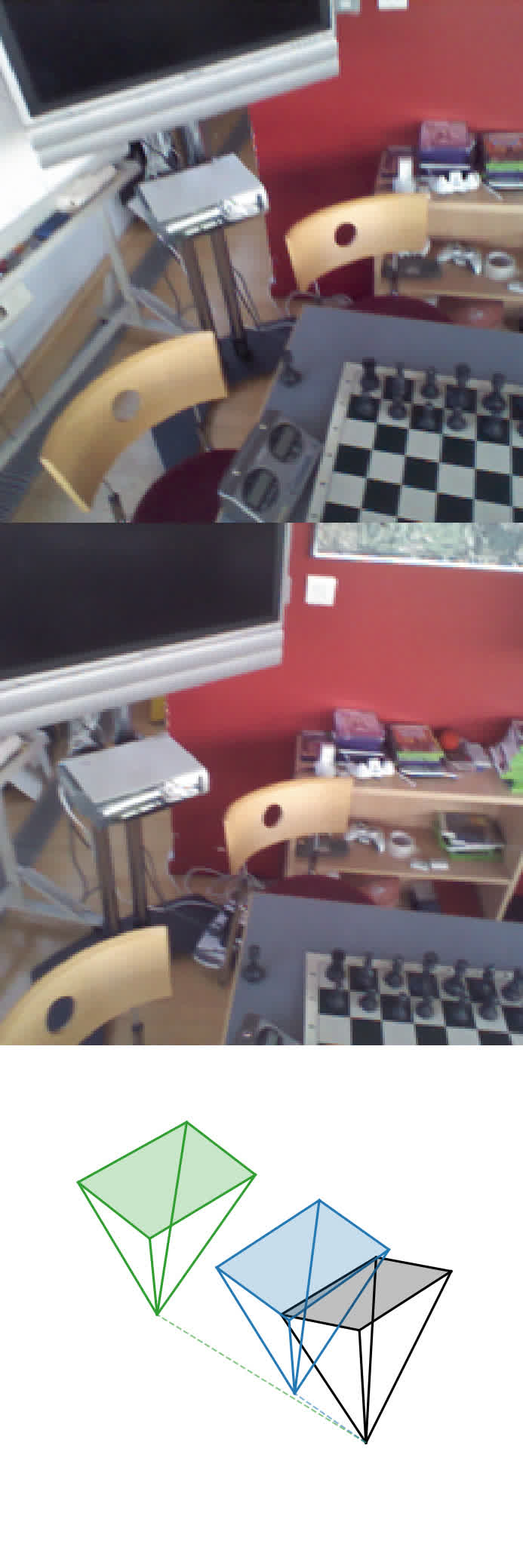
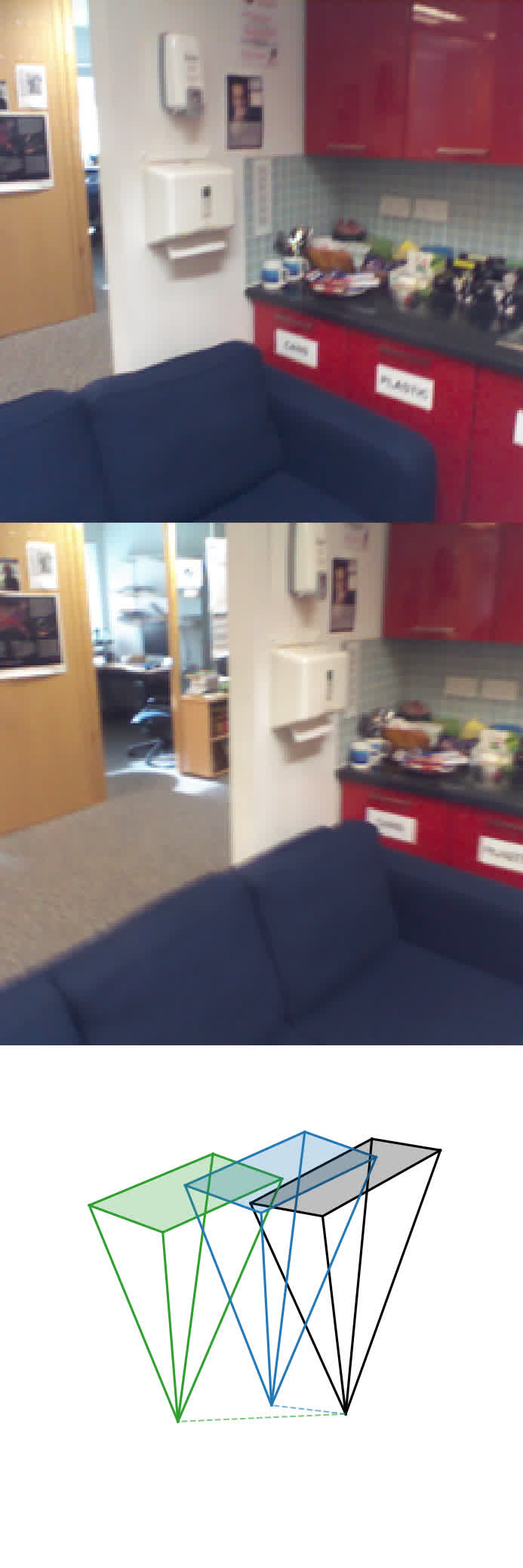
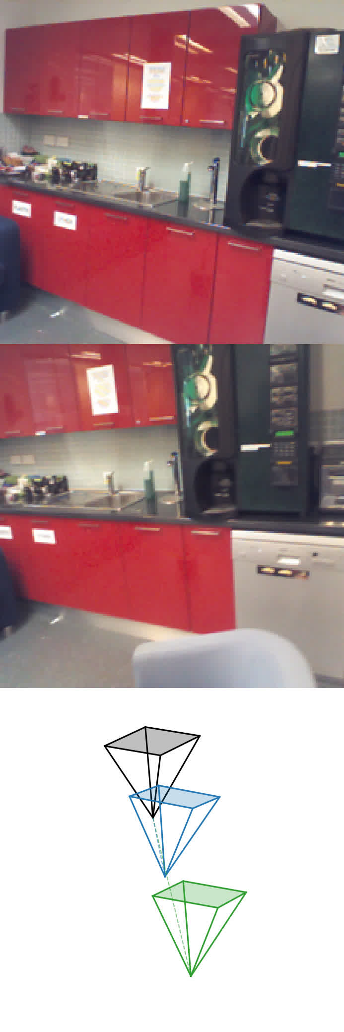
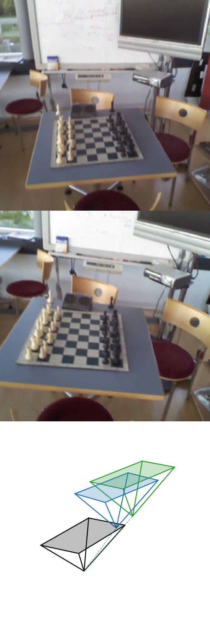
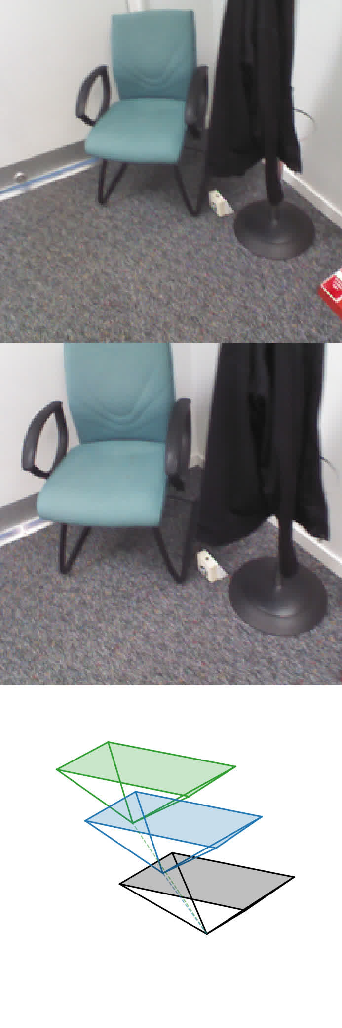
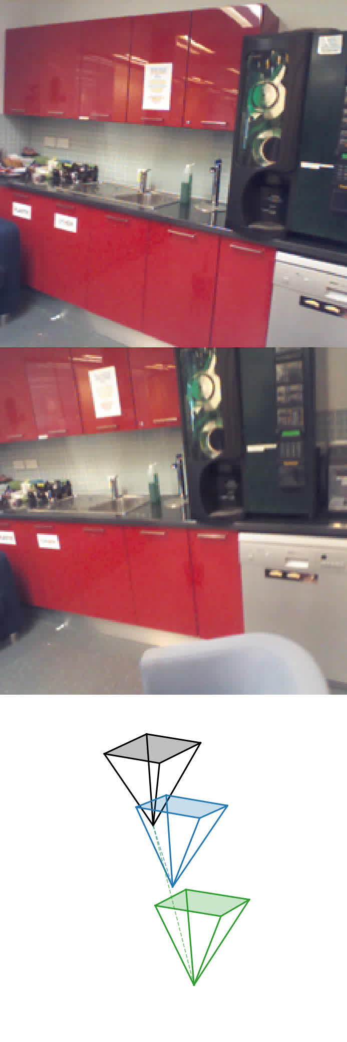
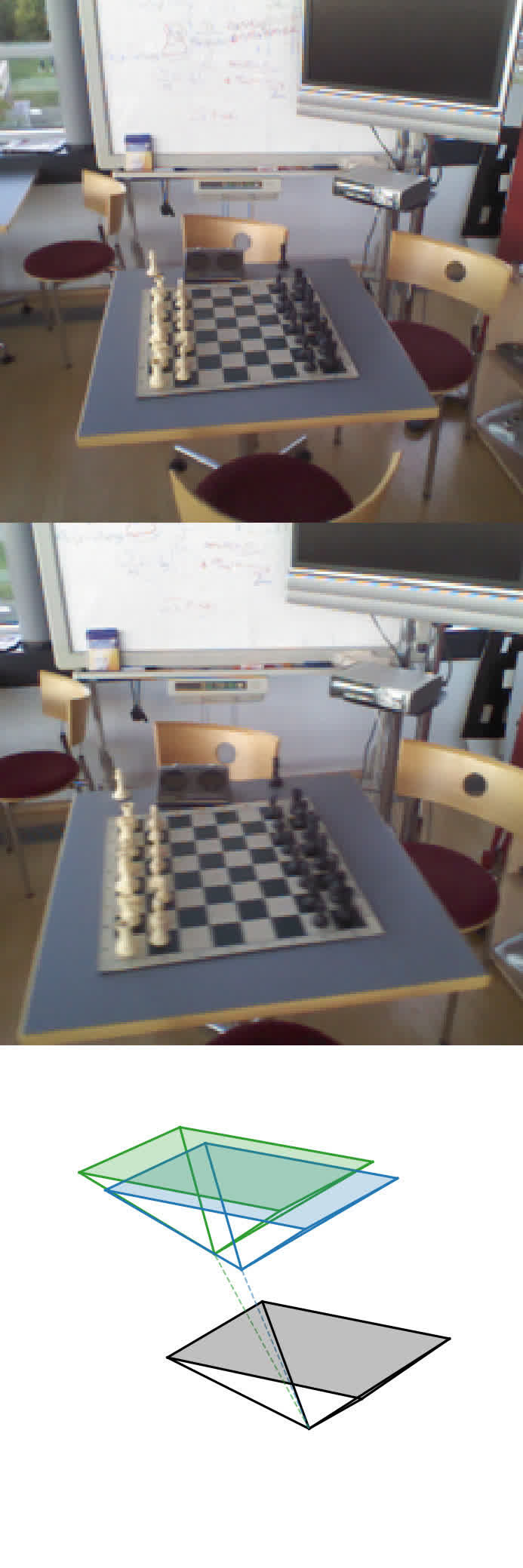
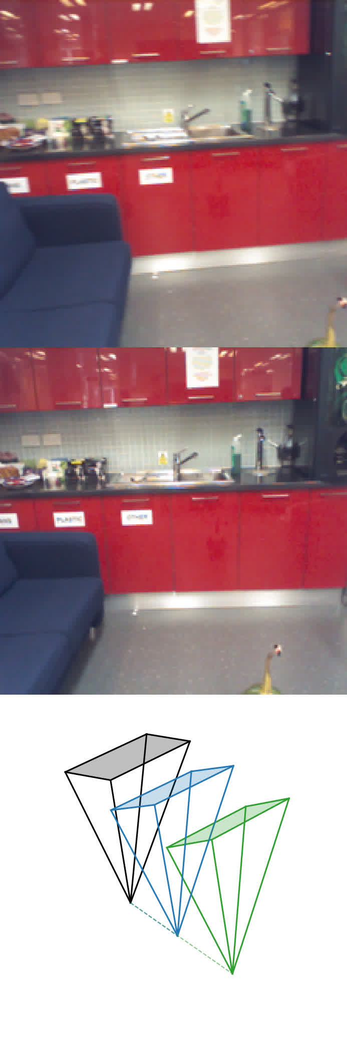
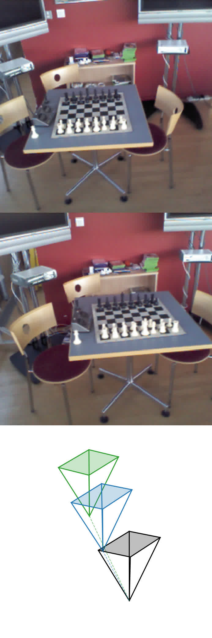
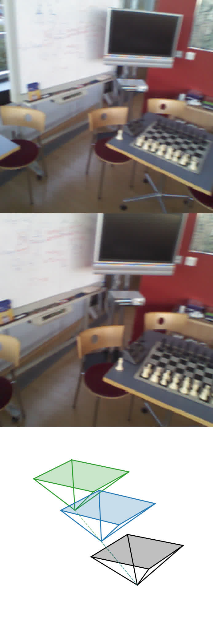
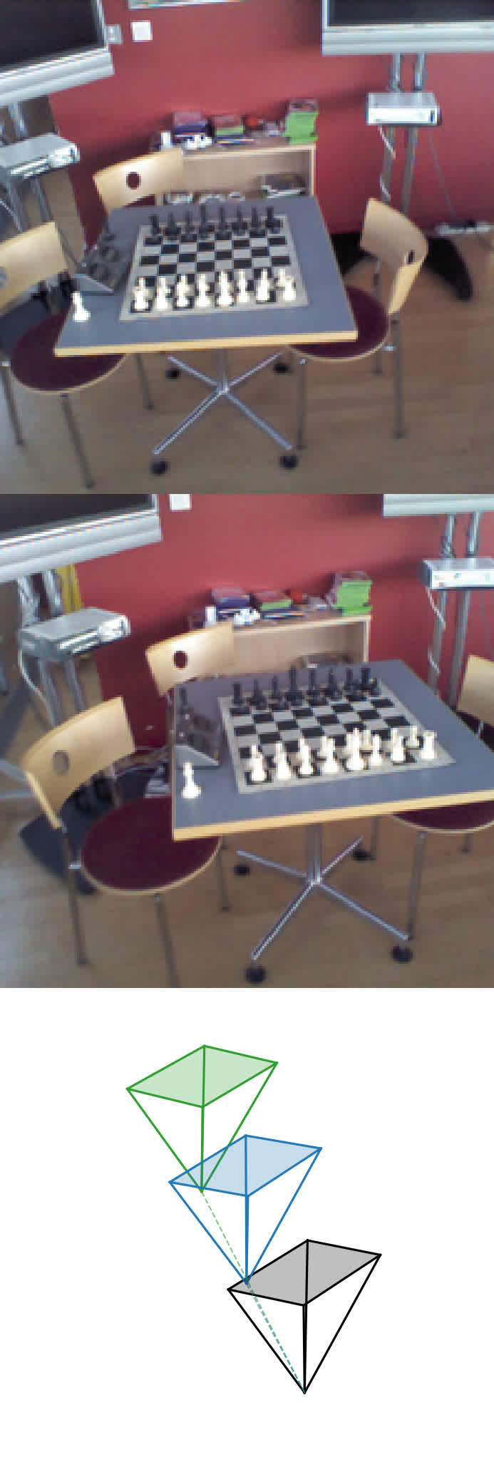
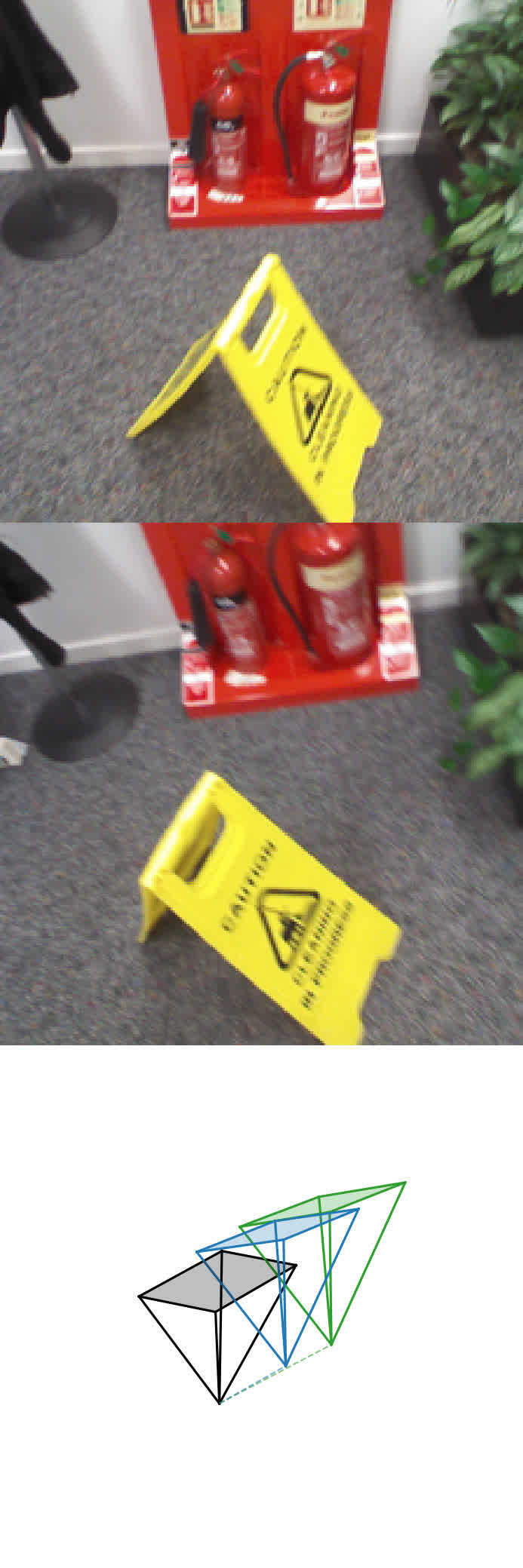
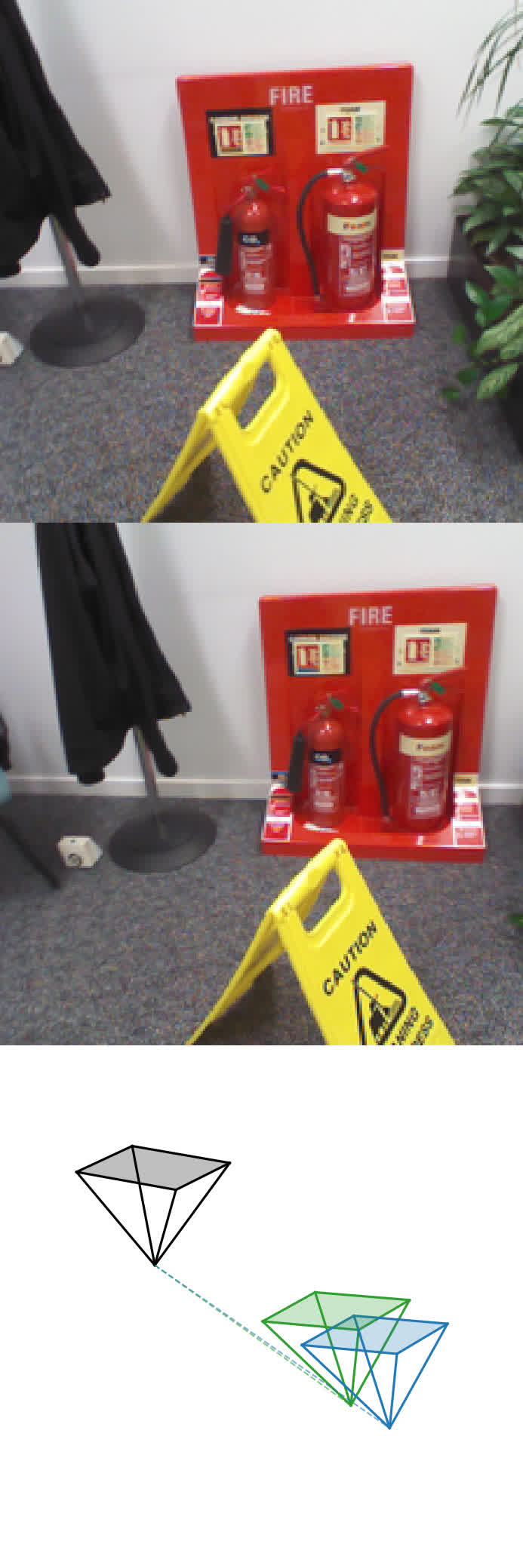
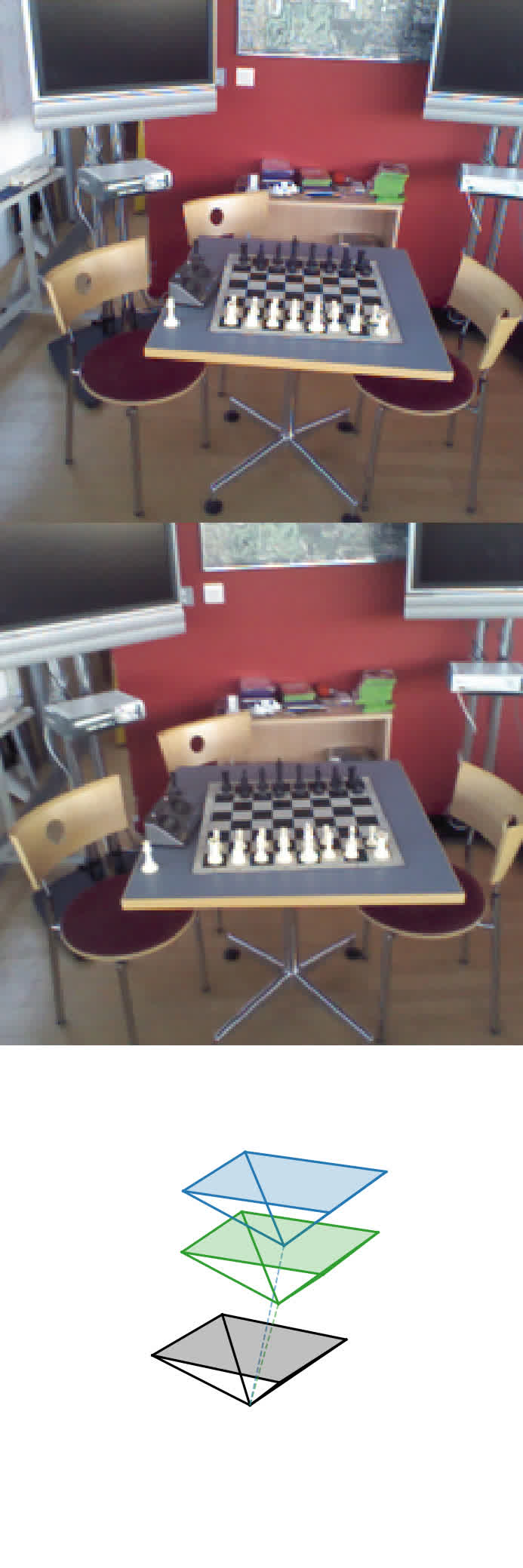
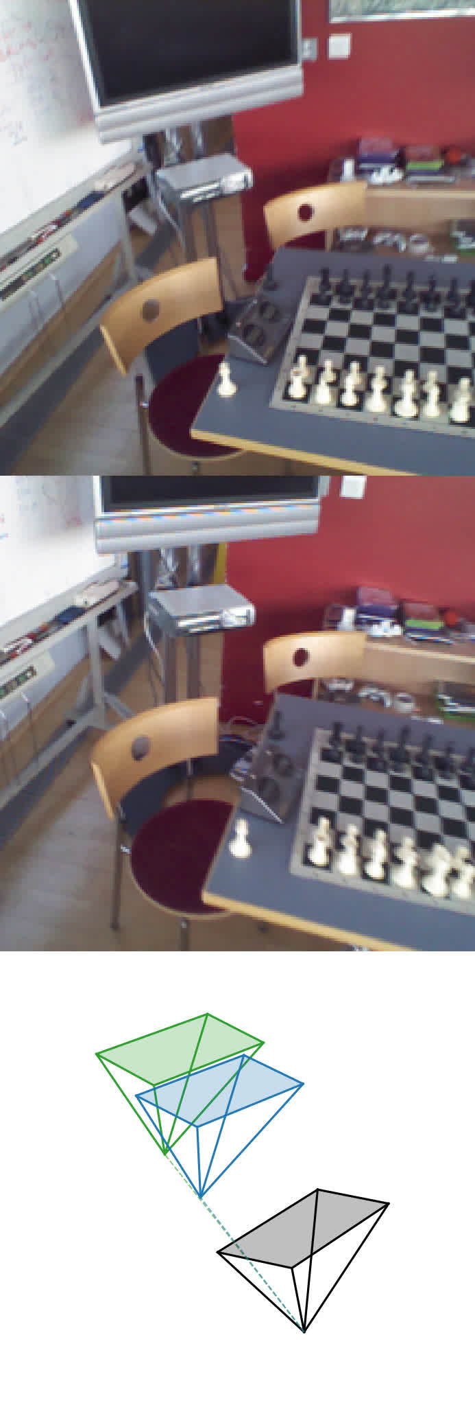
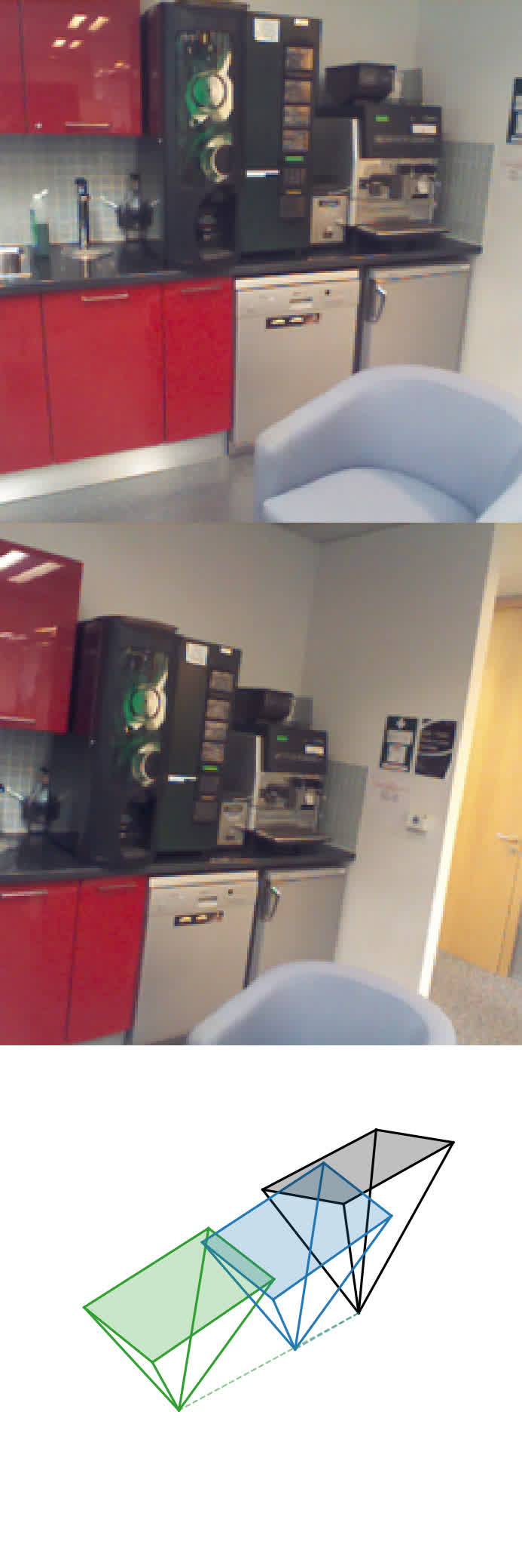
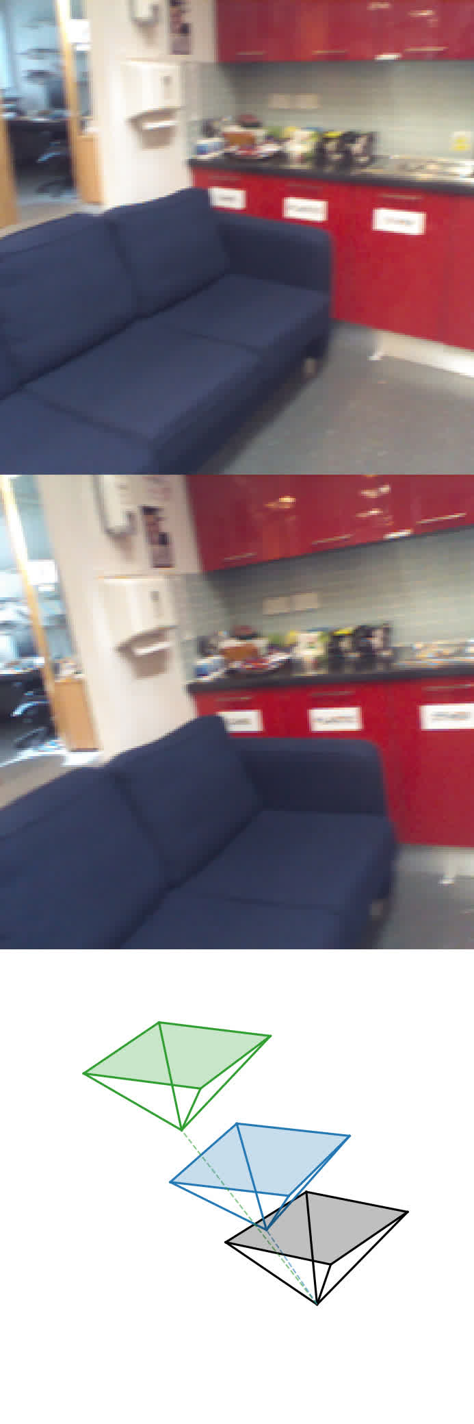
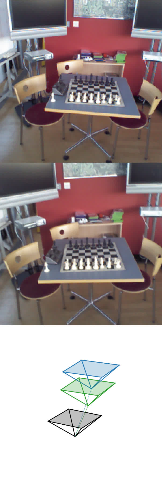
We experiment on the relative pose regression downstream task, where the goal for a given image pair is to predict the relative pose of the camera with respect to a reference view.

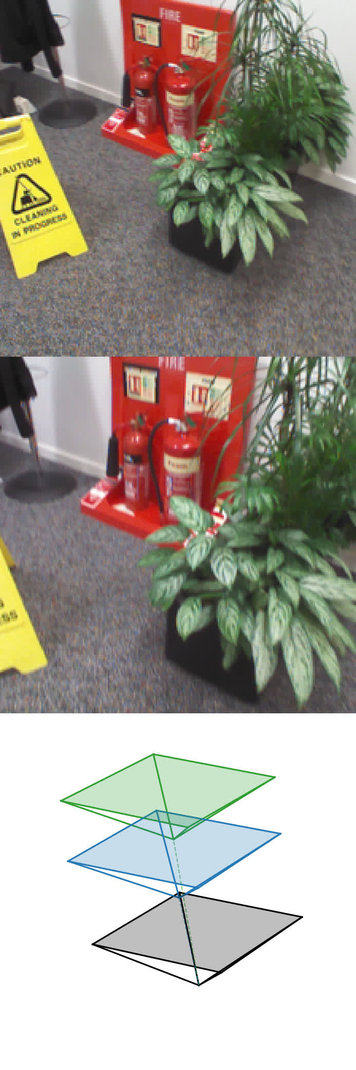
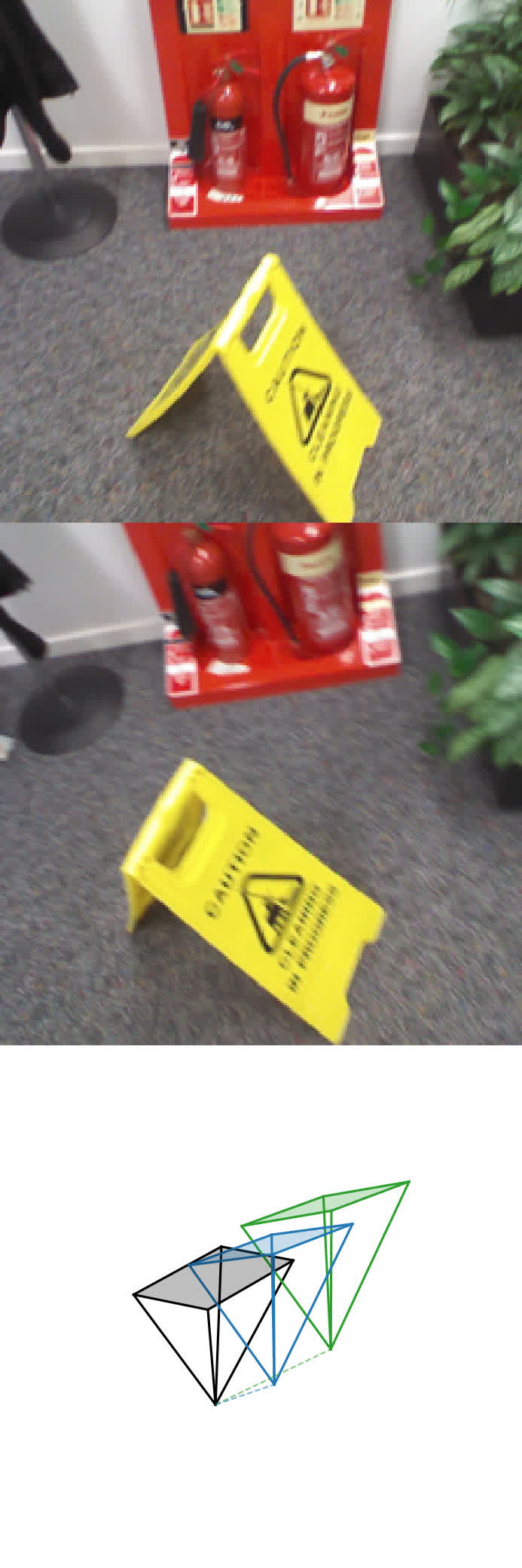
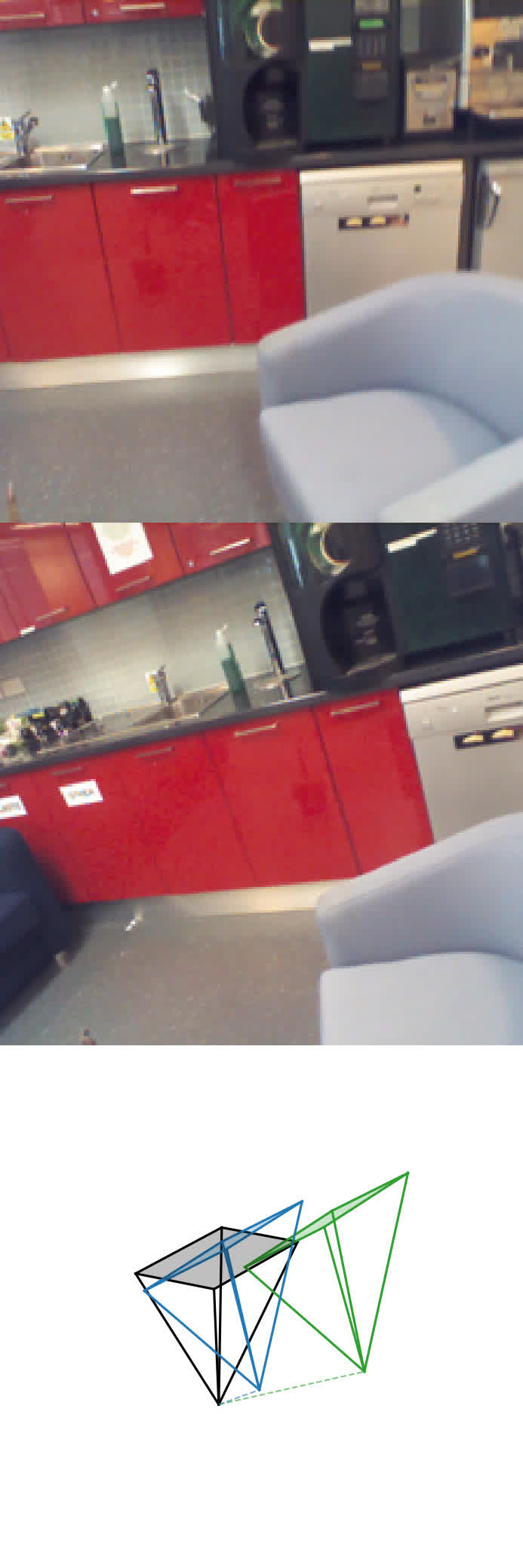
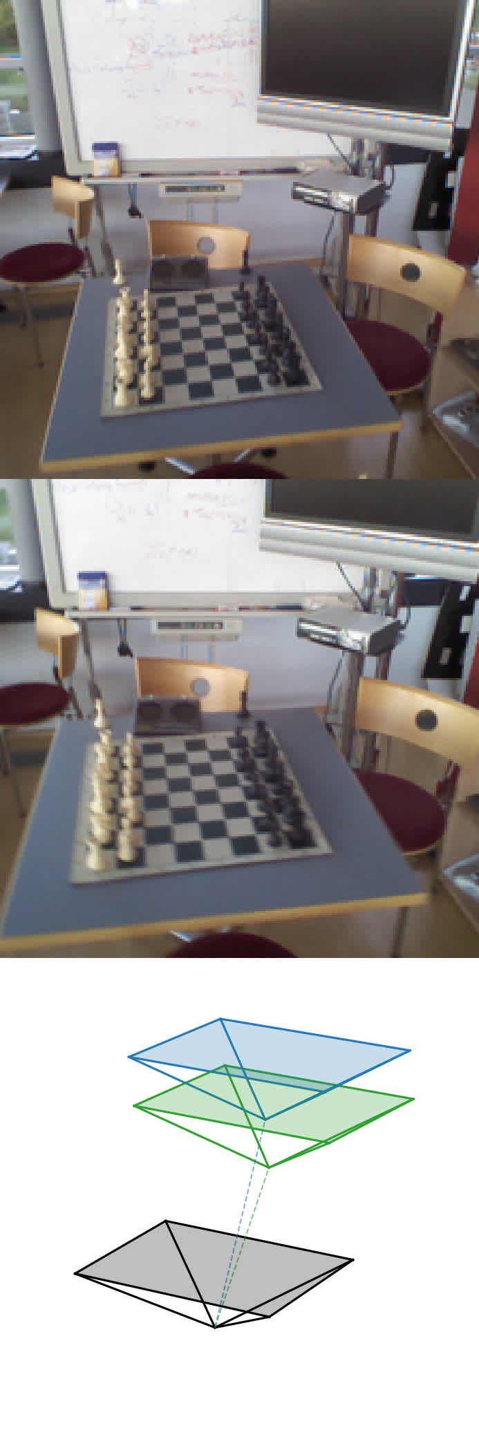
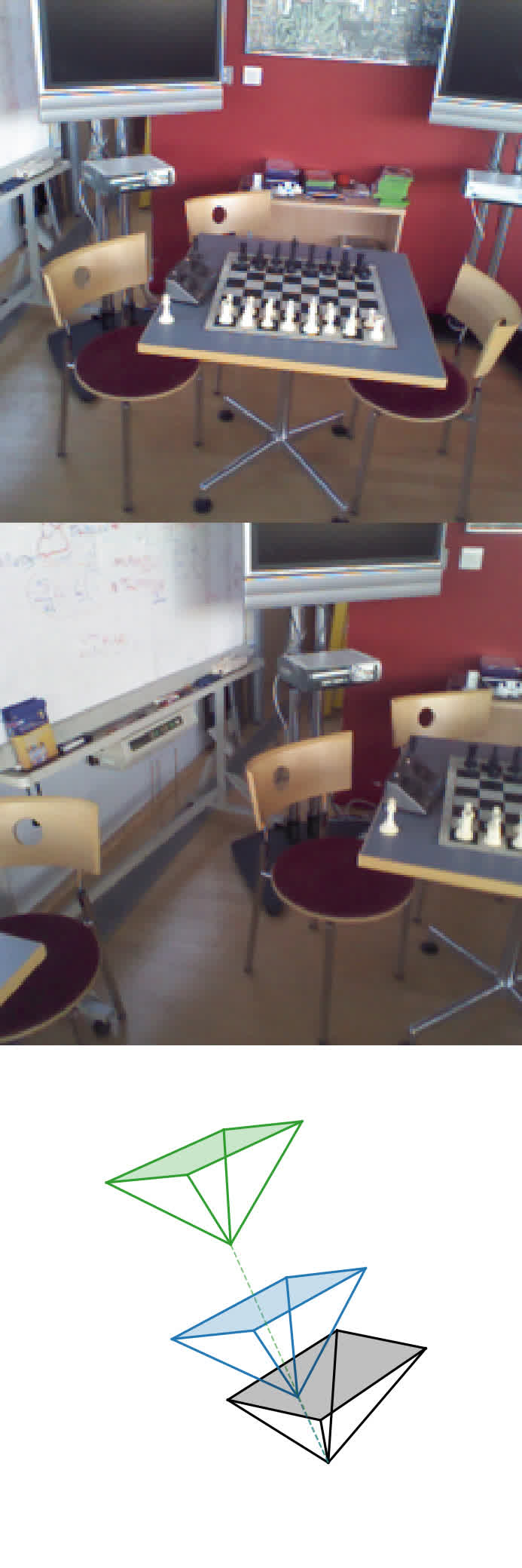
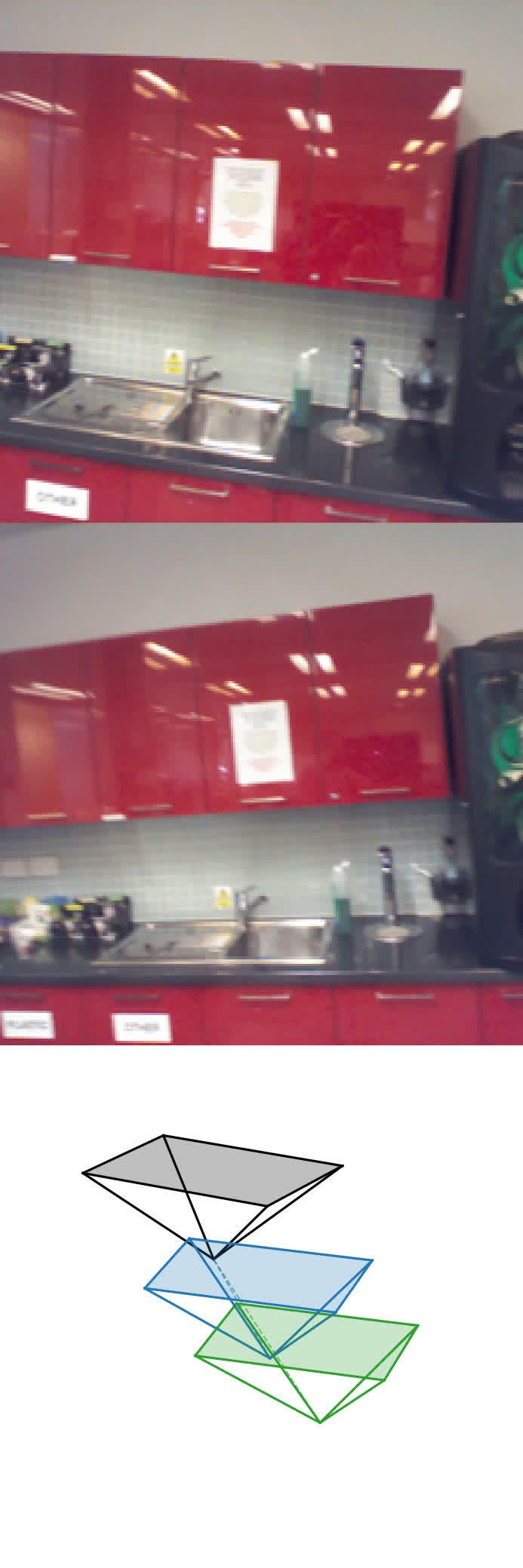
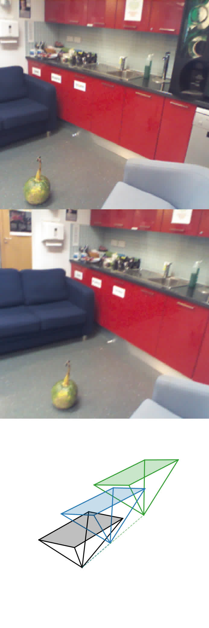
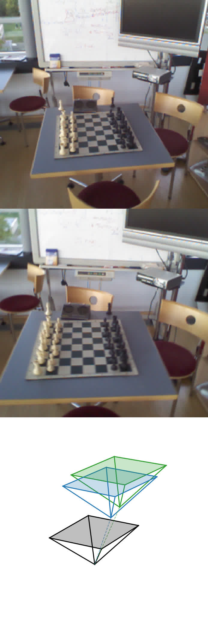
The picture is a carousel. Tap to activate scrolling. The first row shows the reference image, the second row shows the query image, and the third row shows the predicted camera poses: black = reference camera, green = ground truth, blue = our prediction.

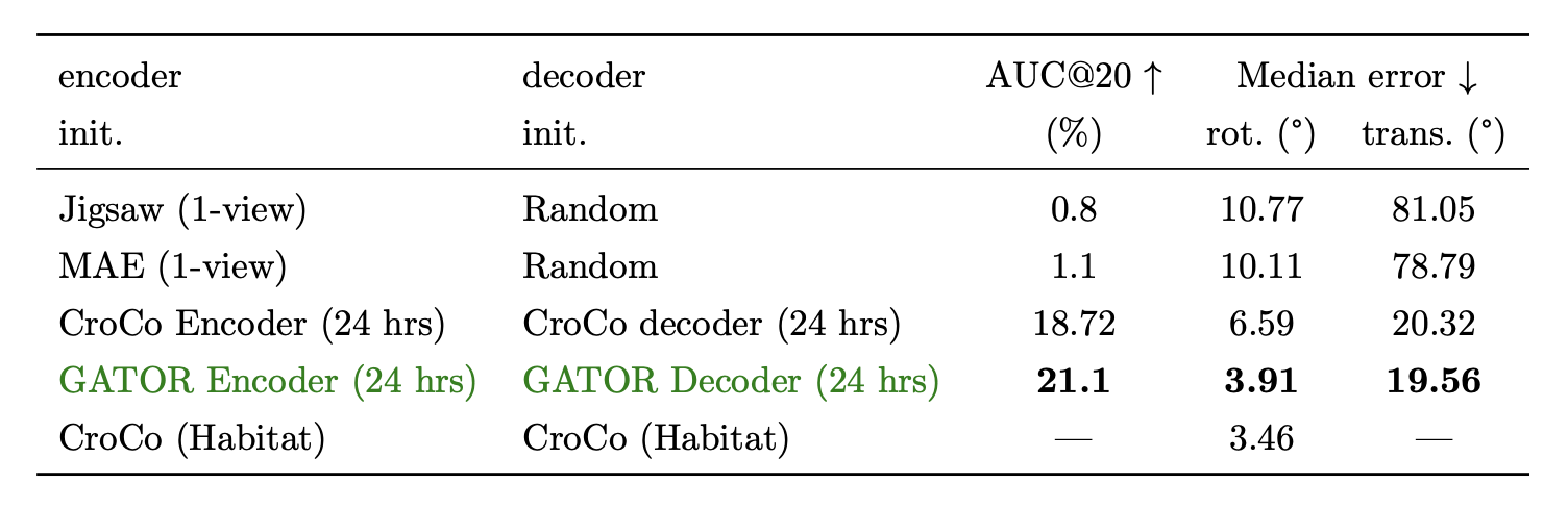
The following table shows the results obtained by fine-tuning the models on the 7-Scenes dataset. The reported performance refers to the test set, evaluated in terms of AUC@20, median rotation error, and median translation angular error.

One-view models (Jigsaw, MAE) struggle to adapt to the pose regression task, while cross-view pretraining leads to substantially better performance. GATOR achieves competitive results compared to CroCo pretrained with comparable compute, demonstrating that its cross-view representations transfer well to relative pose regression. For reference, in the last row of the table we report the results from the original CroCo paper; note that the authors only report median errors, with translation expressed in centimeters rather than angular degrees, so AUC@20 and median translation angular error are not available.

IV-F. Second View Utilization: Tiny Dataset

In this section, we evaluate whether the model uses the second view to solve the task or instead relies solely on the shuffled view. We construct a small dataset of 15 images, sampled from the rendered dataset to keep the domain consistent. We use ChatGPT to edit the images, followed by additional manual refinement in GIMP. For each image \(x_1\), we introduce a modification such that swapping a subset of its patches produces a second image \(x_2\) that still appears realistic, while satisfying \(x_1 \neq x_2\). We then shuffle the patches of \(x_1\) to obtain the shuffled view \(x_s\) and pass the images to the model. If the model produces \[ \operatorname{Gator}(\text{shuffled}=x_s, \text{reference}=x_1) \approx x_1, \qquad \operatorname{Gator}(\text{shuffled}=x_s, \text{reference}=x_2) \approx x_2, \] this indicates that it can use the second view to resolve the ambiguity and correctly solve the task.

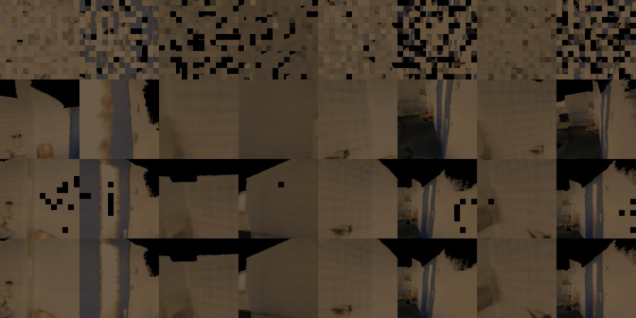
The picture is a carousel. Tap to activate scrolling. Top row is shuffled image before shuffling, middle row is the reference view, and the bottom row is the shuffled view after shuffling.

We observe that the model correctly uses the second view and solves the task for all 30 reference views, corresponding to two reference views for each of the 15 dataset images. Moreover, the prediction accuracy exceeds 98% on the swapped patches. These results suggest that the model learns to use the second view to solve the task, rather than relying on shortcuts. We perform an additional experiment to evaluate the model's reliance on the second view in the appendix (sec E).

IV-G. Cross-Attention Maps

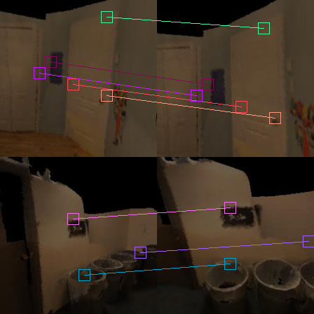
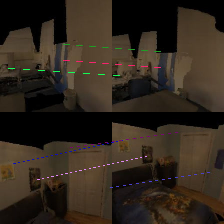
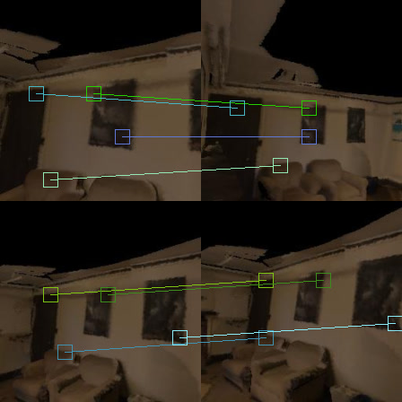
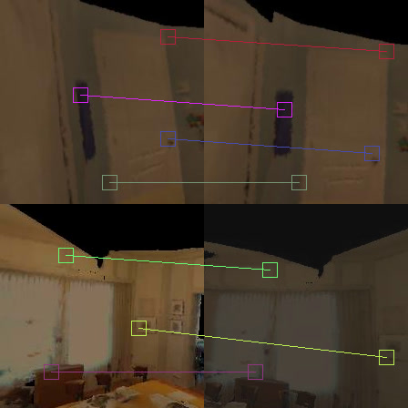
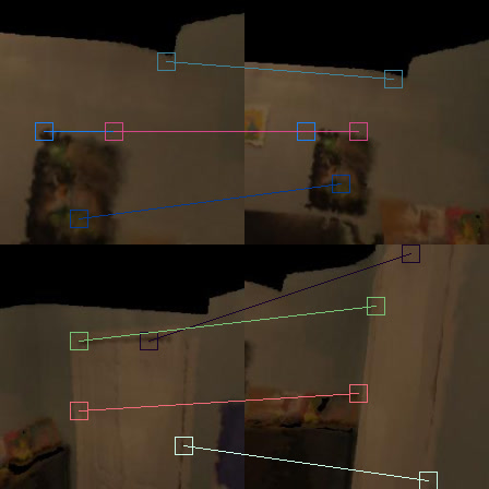
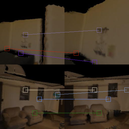
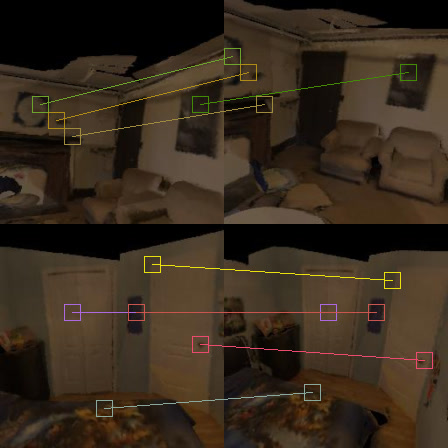
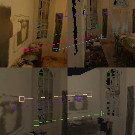
Matching between patches. In each pair one image is shuffled before shuffling and the other is the reference view.

We analyze the cross-attention maps in the model decoder. Surprisingly, we find that the model learns to establish correspondences between patches in the shuffled and reference views without any explicit correspondence supervision. For each token in the shuffled view, we identify the token in the reference view with the highest attention weight and visualize the resulting matches in the carousel above. We use the output of decoder layer 4 for this analysis, as the outputs of later layers do not exhibit clear matching patterns, likely because they focus more on task prediction than on cross-view reasoning.

In this work, we have explored a new pretraining method for multi-view models based on jigsaw puzzle solving. By avoiding pixel-level reconstruction as the pretraining objective, our method is able to adapt effectively to downstream tasks compared to single-view models (MAE, one-view jigsaw) and the multi-view CroCo, when trained with the same compute. We demonstrated that the model learns to use the second view to solve the pretraining task, confirming that the adopted objective encourages cross-view reasoning.
Despite these promising results, several directions remain for future work. (1) Our experiments use ViT-Small-scale models due to limited compute. Future work could evaluate Gator at larger scales and compare it with CroCo and other baselines under similar settings. (2) The current model may assign multiple patches to the same position, resulting in holes in the reconstructed image. While our focus is on pretraining performance rather than optimal jigsaw solving, future work could explore strategies to reduce such duplicate assignments. (3) Finally, our pretraining dataset is synthetic and limited to indoor scenes. Evaluating the method on larger, more diverse datasets, as well as in other domains such as outdoor scenes or other modalities, would be an important direction for further study.

Darcet T, Oquab M, Mairal J, Bojanowski P. Vision transformers need registers. InInternational conference on learning representations 2024 May 31 (Vol. 2024, pp. 2632-2652). https://doi.org/10.48550/arXiv.2309.16588.

Weinzaepfel P, Leroy V, Lucas T, Brégier R, Cabon Y, Arora V, Antsfeld L, Chidlovskii B, Csurka G, Revaud J. Croco: Self-supervised pre-training for 3d vision tasks by cross-view completion. Advances in Neural Information Processing Systems. 2022 Dec 6;35:3502-16. https://doi.org/10.48550/arXiv.2210.10716.

M. Caron, H. Touvron, I. Misra, H. J´egou, J. Mairal, P. Bojanowski, and A. Joulin, “Emerging properties in self-supervised vision transformers,” in Proceedings of the IEEE/CVF international conference on computer vision, 2021, pp. 9650–9660 https://arxiv.org/abs/2104.14294,

K. He, X. Chen, S. Xie, Y. Li, P. Doll´ar, and R. Girshick, “Masked autoencoders are scalable vision learners,” 2021. https://arxiv.org/abs/2111.06377

M. Noroozi and P. Favaro, “Unsupervised learning of visual representations by solving jigsaw puzzles,” 2017. [Online]. Available: https://arxiv.org/abs/1603.09246

M. Noroozi and P. Favaro, “Unsupervised learning of visual representations by solving jigsaw puzzles,” 2017. [Online]. Available: https://arxiv.org/abs/1603.09246

Y. Chen, X. Shen, Y. Liu, Q. Tao, and J. A. K. Suykens, “Jigsaw-vit: Learning jigsaw puzzles in vision transformer,” 2023. [Online]. Available: https://arxiv.org/abs/2207.11971

U. Ahsan, R. Madhok, and I. Essa, “Video jigsaw: Unsupervised learning of spatiotemporal context for video action recognition,” 2018. [Online]. Available: https://arxiv.org/abs/1808.07507

Z. Song, Z. Hu, and R. Hong, “Grid jigsaw representation with clip: a new perspective on image clustering,” Multimedia Systems, vol. 31, no. 2, Feb. 2025. [Online]. Available: http://dx.doi.org/10.1007/s00530-025-01703-x

P. Wu, Y. Zhang, H. Diao, B. Li, L. Lu, and Z. Liu, “Visual jigsaw post-training improves mllms,” 2025. [Online]. Available: https://arxiv.org/abs/2509.25190

D. Nordstr¨om, J. Edstedt, F. Kahl, and G. B¨okman, “Mum: Multi-view masked image modeling for 3d vision,” 2025. [Online]. Available: https://arxiv.org/abs/2511.17309

A. Ablation on Jigsaw Objective

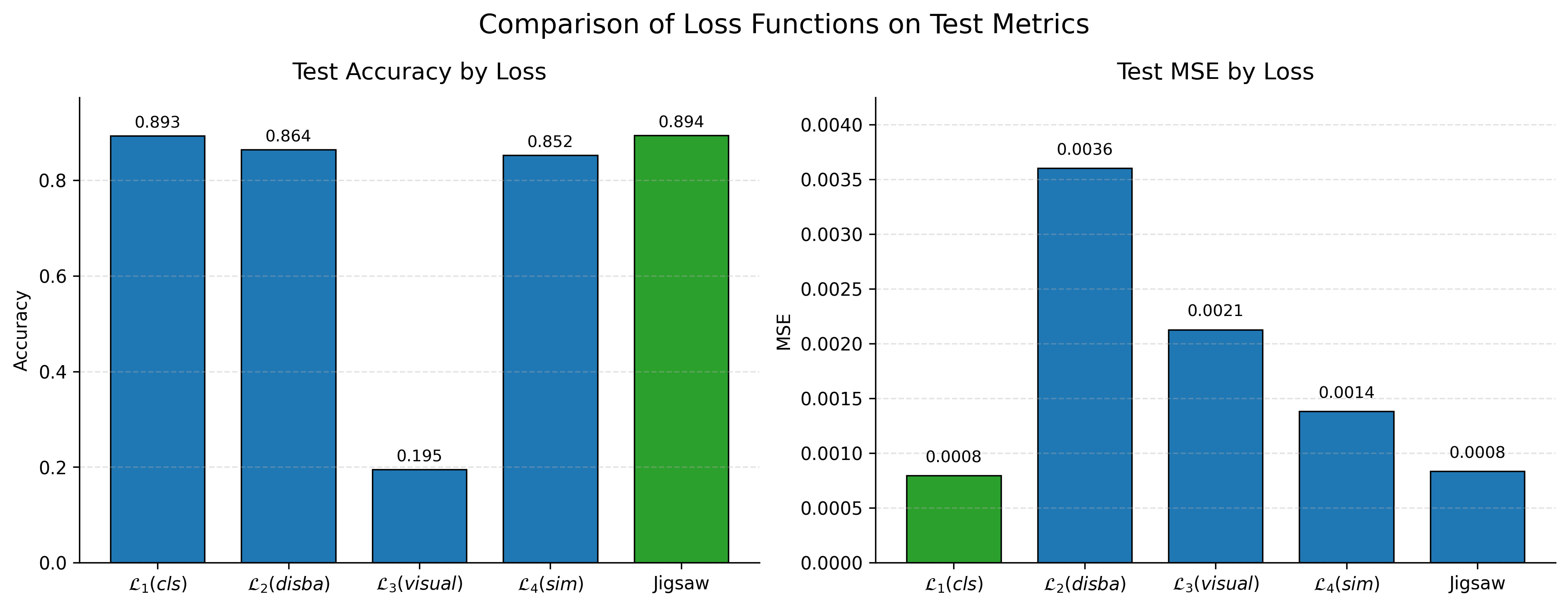
We train the model using the different jigsaw objectives described in Section III-B and compare their performance on the pretraining task. Due to computational constraints, we use a ViT-Tiny model and train each variant for 12 hours on a single V100 GPU. We follow the same training setup as described in Section IV-A. For each objective, we tune the learning rate on the validation set and use the best-performing learning rate to train the final model.

Regardless of the learning rate, the model trained with the visual loss does not converge within 12 hours and achieves the worst performance. We attribute this to the greater complexity of the visual objective, which requires the model to infer both patch positions and their contributions to the reconstructed image.

The classification objective achieves the best accuracy and MSE, so we use it in our finetuning experiments. The distance-based objective achieves the second-best performance, suggesting that it may be a viable alternative to the classification objective. One advantage of the distance-based objective is that it encodes a notion of similarity between positions: nearby positions are treated as more similar than distant ones. The similarity loss performs better than the visual loss but worse than the classification and distance-based objectives. This may be because replacing the one-hot target with a soft target distribution makes the task more difficult.

B. Ablation on Masking Ratios

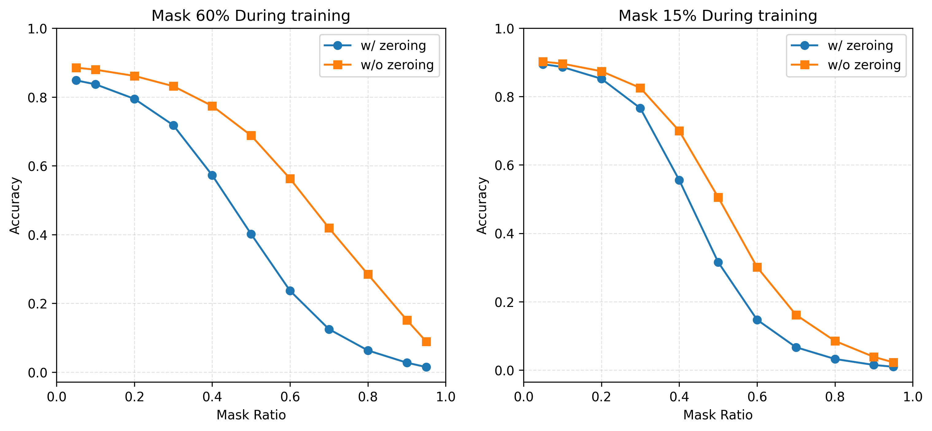
We perform a small ablation study to evaluate the effectiveness of randomly masking a portion of the shuffled-view patches during training. We train two models with the same architecture and training setup, varying only the masking ratio. One model is trained with approximately 60% of shuffled-view patches masked out, referred to as model-60%, while the other is trained with approximately 15% masking, referred to as model-15%. We then compare their performance using the same evaluation strategy as in Section IV-F.

The figure shows that the performance curves with and without zeroing the reference view are closer for model-15%. We further evaluate both models on the Tiny Dataset and observe that model-15% achieves approximately 91% accuracy on swapped patches, whereas model-60% achieves approximately 98% accuracy.

These results suggest that the model trained with 15% masking relies less on the reference view to solve the task. This supports the effectiveness of our strategy of masking a substantial portion of shuffled-view patches during training to encourage the model to utilize the reference view.

C. Classification Examples

It this section we provide additional visualizations of the classification predictions of our model on ImageNet validation samples. We selected 15 labels from the ImageNet validation set (50,000 images). The left column shows the input image with its ground-truth class; the right column shows the top-1 prediction of each model, highlighted green ✓ if correct and red ✗ if wrong, along with the softmax confidence. Slides advance automatically; click any arrow or dot to take control.

D. More Optical Flow Examples

It this section we provide additional visualizations of the optical flow predictions of our model on MPI-Sintel. The picture is a carousel. Tap to activate scrolling. The first row shows the input frames, the second row shows the ground truth for optical flow, the third row shows Gator's prediction.

E. Second View Utilization: Zero Reference

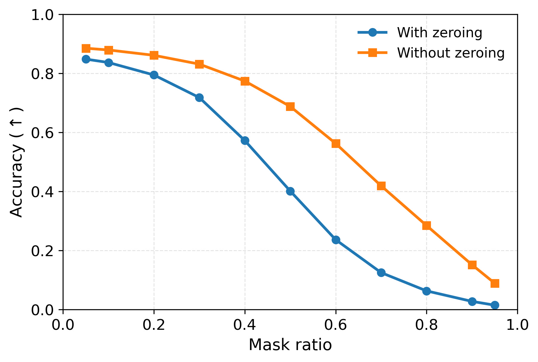
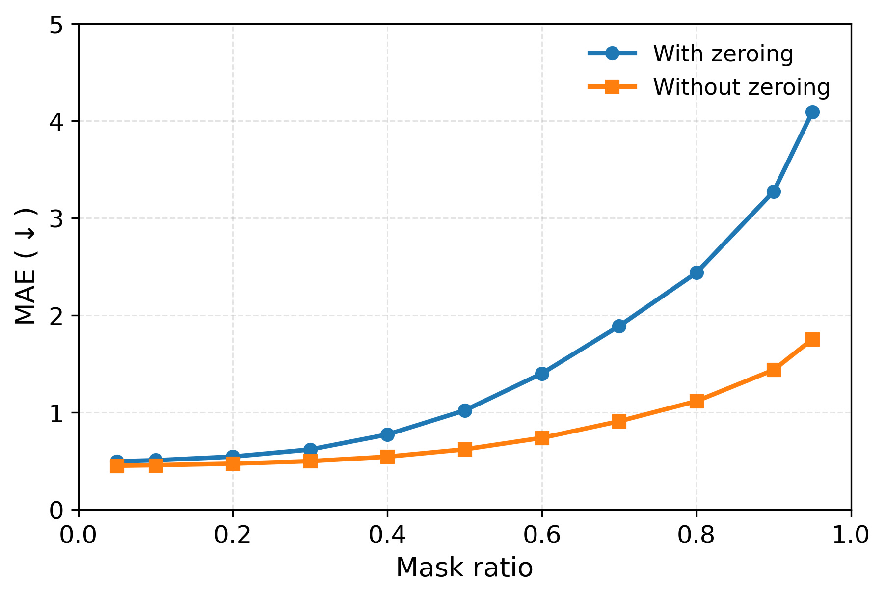
In this section, we evaluate whether the model uses the second view to solve the task or instead relies solely on the shuffled view. We compare performance when the model is given the true reference image against performance when the reference image is replaced with a zero image. A substantial performance drop in the latter setting would indicate that the model relies on the reference view to solve the task.

As shown in the plots above, providing the true reference view improves model performance, particularly when a moderate fraction of the shuffled patches is masked. The largest improvement is observed when 60% of the shuffled patches are masked. One notable behavior is that the two settings yield similar performance when the full shuffled image is available. This can be explained by the fact that patch positions are easier to infer when all shuffled patches are present. In contrast, performance drops when a large fraction of patches is masked. This is likely because our model does not use RoPE for shuffled-view patches, making it more difficult to infer their relative positions with respect to the reference view.